13
Transparency
Imagine that you are a model validator in the model risk management department at JCN Corporation, the (fictional) information technology company undergoing an enterprise transformation first encountered in Chapter 7. In addition to using machine learning for estimating the skills of its employees, JCN Corporation is rolling out machine learning in another human resources effort: proactive retention. Using historical employee administrative data, JCN Corporation is developing a system to predict employees at risk of voluntarily resigning in the next six months and offering incentives to retain them. The data includes internal corporate information on job roles and responsibilities, compensation, market demand for jobs, performance reviews, promotions, and management chains. JCN Corporation has consent to use the employee administrative data for this purpose through employment contracts. The data was made available to JCN Corporation’s data science team under institutional control after a syntactic anonymity transformation was performed.
The team has developed several attrition prediction models using different machine learning algorithms, keeping accuracy, fairness, distributional robustness, adversarial robustness, and explainability as multiple goals. If the attrition prediction models are fair, the proactive retention system could make employment at JCN Corporation more equitable than it is right now. The project has moved beyond the problem specification, data understanding, data preparation, and modeling phases of the development lifecycle and is now in the evaluation phase.
“The full cycle of a machine learning project is not just modeling. It is finding the right data, deploying it, monitoring it, feeding data back [into the model], showing safety—doing all the things that need to be done [for a model] to be deployed. [That goes] beyond doing well on the test set, which fortunately or unfortunately is what we in machine learning are great at.”
—Andrew Ng, computer scientist at Stanford University
Your job as the model validator is to test out and compare the models to ensure at least one of them is safe and trustworthy before it is deployed. You also need to obtain buy-in from various parties before you can sign your name and approve the model’s deployment. To win the support of internal JCN Corporation executives and compliance officers, external regulators,[1] and members of a panel of diverse employees and managers within the company you’ll assemble, you need to provide transparency by communicating not only the results of independent tests you conduct, but also what happened in the earlier phases of the lifecycle. (Transparent reporting to the general public is also something you should consider once the model is deployed.) Such transparency goes beyond model interpretability and explainability because it is focused on model performance metrics and their uncertainty characterizations, various pieces of information about the training data, and the suggested uses and possible misuses of the model.[2] All of these pieces of information are known as facts.
Not all of the various consumers of your transparent reporting are looking for the same facts or the same level of detail. Modeling tasks besides predicting voluntary attrition may require different facts. Transparency has no one-size-fits-all solution. Therefore, you should first run a small design exercise to understand which facts and details are relevant for the proactive retention use case and for each consumer, and the presentation style preferred by each consumer.[3] (Such an exercise is related to value alignment, which is elaborated upon in Chapter 14.) The artifact that ultimately presents a collection of facts to a consumer is known as a factsheet. After the design exercise, you can be off to the races with creating, collecting, and communicating information about the lifecycle.
You are shouldering a lot of responsibility, so you don’t want to perform your job in a haphazard way or take any shortcuts. To enable you to properly evaluate and validate the JCN Corporation voluntary resignation models and communicate your findings to various consumers, this chapter teaches you to:
§ create factsheets for transparent reporting,
§ capture facts about the model purpose, data provenance, and development steps,
§ conduct tests that measure the probability of expected harms and the possibility of unexpected harms to generate quantitative facts,
§ communicate these test result facts and their uncertainty, and
§ defend your efforts against people who are not inclined to trust you.
You’re up to the task padawan, so let’s start equipping you with the tools you need.
13.1 Factsheets
Transparency should reveal several kinds of facts that come from different parts of the lifecycle.[4] From the problem specification phase, it is important to capture the goals, intended uses, and possible misuses of the system along with who was involved in making those decisions (e.g. were diverse voices included?). From the data understanding phase, it is important to capture the provenance of the data, including why it was originally collected. From the data preparation phase, it is important to catalog the data transformations and feature engineering steps employed by the data engineers and data scientists, as well as any data quality analyses that were performed. From the modeling phase, it is important to understand what algorithmic choices were made and why, including which mitigations were employed. From the evaluation phase, it is important to test for trust-related metrics and their uncertainties (details are forthcoming in the next section). Overall, there are two types of facts for you to transparently report: (1) (qualitative) knowledge from inside a person’s head that must be explicitly asked about, and (2) data, processing steps, test results, models, or other artifacts that can be grabbed digitally.
How do you get access to all this information coming from all parts of the machine learning development lifecycle and from different personas? Wouldn’t it be convenient if it were documented and transparently reported all along? Because of the tireless efforts of your predecessors in the model risk management department, JCN Corporation has instrumented the entire lifecycle with a mandatory tool that manages machine learning development by creating checklists and pop-up reminders for different personas to enter qualitative facts at the time they should be top-of-mind for them. The tool also automatically collects and version-controls digital artifacts as facts as soon as they are generated. Let’s refer to the tool as fact flow, which is shown in Figure 13.1.
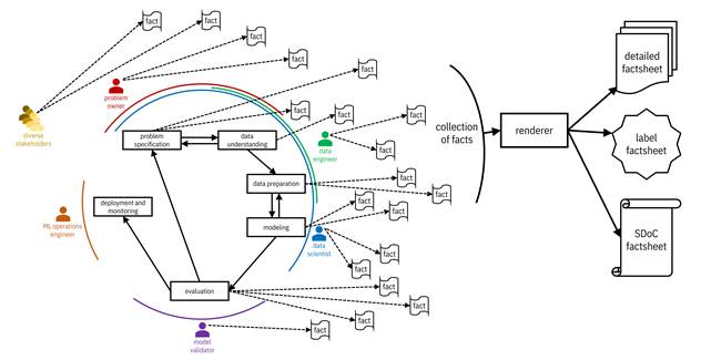
Figure 13.1. The fact flow captures qualitative and quantitative facts generated by different people and processes throughout the machine learning development lifecycle and renders them into factsheets appropriate for different consumers. Accessible caption. Facts from people and technical steps in the development lifecycle go into a renderer which may output a detailed factsheet, a label factsheet, or a SDoC factsheet.
Since machine learning is a general purpose technology (recall the discussion in Chapter 1), there is no universal set of facts that applies to all machine learning models irrespective of their use and application domain. The facts to validate the machine learning systems for m-Udhār Solar, Unconditionally, ThriveGuild, and Wavetel (fictional companies discussed in previous chapters) are not exactly the same; more precision is required.[5] Moreover, the set of facts that make it to a factsheet and their presentation depends on the consumer. As the model validator, you need a full dump of all the facts. You should adjust the factsheet to a summary label, document, or presentation slides for personas who, to overcome their cognitive biases, need fewer details. You should broadly disseminate simpler factsheets among JCN Corporation managers (decision makers), employees (affected users), and the general public who yearn for transparency. You will have determined the set of facts, their level of detail, and their presentation style for different personas through your initial design exercise. Fact flow has a renderer for you to create different factsheet presentations.
You should also sign and release a factsheet rendered as a supplier’s declaration of conformity (SDoC) for external regulators. An SDoC is a written assurance that a product or service conforms to a standard or technical regulation. Your declaration is based on your confidence in the fact flow tool and the inspection of the results you have conducted.[6] Conformity is one of several related concepts (compliance, impact, and accountability), but different from each of them.[7] Conformity is abiding by specific regulations whereas compliance is abiding by broad regulatory frameworks. Conformity is a statement on abiding by regulations at the current time whereas impact is abiding by regulations into an uncertain future. Conformity is a procedure by which to show abidance whereas accountability is a responsibility to do so. As such, conformity is the narrowest of definitions and is the one that forms the basis for the draft regulation of high-risk machine learning systems in the European Economic Area and may become a standard elsewhere too. Thus SDoCs represent an up-and-coming requirement for machine learning systems used in high-stakes decision making, including proactive retention at JCN Corporation.
“We really need standards for what an audit is.”
—Rumman Chowdhury, machine learning ethicist at Twitter
13.2 Testing for Quantitative Facts
Many quantitative facts come from your model testing in the evaluation phase. Testing a machine learning model seems easy enough, right? The JCN Corporation data scientists already obtained good accuracy numbers on an i.i.d. held-out data set, so what’s the big deal? First, you cannot be sure that the data scientists completely isolated their held-out data set and didn’t incur any leakage into modeling.[8] As the model validator, you can ensure such isolation in your testing.
Importantly, testing machine learning systems is different from testing other kinds of software systems.[9] Since the whole point of machine learning systems is to generalize from training data to label new unseen input data points, they suffer from the oracle problem: not knowing what the correct answer is supposed to be for a given input.[10] The way around this problem is not by looking at a single employee’s input data point and examining its corresponding output attrition prediction, but by looking at two or more variations that should yield the same output. This approach is known as using metamorphic relations.
For example, a common test for counterfactual fairness (described in Chapter 10) is to input two data points that are the same in every way except having different values of a protected attribute. If the predicted label is not the same for both of them, the test for counterfactual fairness fails. The important point is that the actual predicted label value (will voluntarily resign/won’t voluntarily resign) is not the key to the test, but whether that predicted value is equal for both inputs. As a second example for competence, if you multiply a feature’s value by a constant in all training points, train the model, and then score a test point that has been scaled by the same constant, you should get the same prediction of voluntary resignation as if you had not done any scaling at all. In some other application involving semi-structured data, a metamorphic relation for an audio clip may be to speed it up or slow it down while keeping the pitch the same. Coming up with such metamorphic relations requires ingenuity; automating this process is an open research question.
In addition to the oracle problem of machine learning, there are three factors you need to think about that go beyond the typical testing done by JCN Corporation data scientists while generating facts:
1. testing for dimensions beyond accuracy, such as fairness, robustness, and explainability,
2. pushing the system to its limits so that you are not only testing average cases, but also covering edge cases, and
3. quantifying aleatoric and epistemic uncertainty around the test results.
Let’s look into each of these three concerns in turn.
13.2.1 Testing for Dimensions of Trustworthiness
If you’ve reached this point in the book, it will not surprise you that testing for accuracy (and related performance metrics described in Chapter 6) is not sufficient when evaluating machine learning models that are supposed to be trustworthy. You also need to test for fairness using metrics such as disparate impact ratio and average odds difference (described in Chapter 10), adversarial robustness using metrics such as empirical robustness and CLEVER score (described in Chapter 11), and explainability using metrics such as faithfulness (described in Chapter 12).[11] You also need to test for accuracy under distribution shifts (described in Chapter 9). Since the JCN Corporation data science team has created multiple attrition prediction models, you can compare the different options. Once you have computed the metrics, you can display them in the factsheet as a table such as Table 13.1 or in visual ways to be detailed in Section 13.3 to better understand their domains of competence across dimensions of trustworthiness. (Remember that domains of competence for accuracy were a main topic of Chapter 7.)
Table 13.1. Result of testing several attrition models for multiple trust-related metrics.
|
Model |
Accuracy |
Accuracy with Distribution Shift |
Disparate Impact Ratio |
Empirical Robust-ness |
Faithful-ness |
|
logistic regression |
|
|
|
|
|
|
neural network |
|
|
|
|
|
|
decision forest (boosting) |
|
|
|
|
|
|
decision forest (bagging) |
|
|
|
|
|
In these results, the decision forest with boosting has the best accuracy and robustness to distribution shift, but the poorest adversarial robustness, and poor fairness and explainability. In contrast, the logistic regression model has the best adversarial robustness and explainability, while having poorer accuracy and distributional robustness. None of the models have particularly good fairness (disparate impact ratio), and so the data scientists should go back and do further bias mitigation. The example emphasizes how looking only at accuracy leaves you with blind spots in the evaluation phase. As the model validator, you really do need to test for all the different metrics.
13.2.2 Generating and Testing Edge Cases
The primary way to test or audit machine learning models is by feeding in data from different employees and looking at the output attrition predictions that result.[12] Using a held-out dataset with the same probability distribution as the training data will tell you how the model performs in the average case. This is how to estimate empirical risk (the empirical approximation to the probability of error), and thus the way to test for the first of the two parts of safety: the risk of expected harms. Similarly, using held-out data with the same probability distribution is common practice (but not necessary) to test for fairness and explainability. Testing for distributional robustness, by definition however, requires input data points drawn from a probability distribution different from the training data. Similarly, computing empirical adversarial robustness involves creating adversarial example employee features as input.
In Chapter 11, you have already learned how to push AI systems to their limits using adversarial examples. These adversarial examples are test cases for unexpected, worst-case harms that go beyond the probability distribution of the training and held-out datasets. And in fact, you can think about crafting adversarial examples for fairness and explainability as well as for accuracy.[13] Another way to find edge cases in machine learning systems is by using a crowd of human testers who are challenged to ‘beat the machine.’[14] They get points in a game for coming up with rare but catastrophic data points.
Importantly, the philosophy of model validators such as yourself who are testing the proactive retention system is different from the philosophy of malicious actors and ‘machine beaters.’ These adversaries need to succeed just once to score points, whereas model validators need to efficiently generate test cases that have good coverage and push the system from many different sides. You and other model validators have to be obsessed with failure; if you’re not finding flaws, you have to think that you’re not trying hard enough.[15] Toward this end, coverage metrics have been developed for neural networks that measure if every neuron in the model has been tested. However, such coverage metrics can be misleading and do not apply to other kinds of machine learning models.[16] Developing good coverage metrics and test case generation algorithms to satisfy those coverage metrics remains an open research area.
13.2.3 Uncertainty Quantification
As you evaluate and validate proactive retention models for JCN Corporation, testing gives you estimates of the different dimensions of trust as in Table 13.1. But as you’ve learned throughout the book, especially Chapter 3, uncertainty is everywhere, including in those test results. By quantifying the uncertainty of trust-related metrics, you can be honest and transparent about the limitations of the test results. Several different methods for uncertainty quantification are covered in this section, summarized in Figure 13.2.
“I can live with doubt and uncertainty and not knowing. I think it’s much more interesting to live not knowing than to have answers which might be wrong.”
—Richard Feynman, physicist at California Institute of Technology
The
total predictive uncertainty includes both aleatoric and epistemic uncertainty.
It is indicated by the score for well-calibrated classifiers (remember the
definition of calibration, Brier score, and calibration loss[17]
from Chapter 6). When the attrition prediction classifier is well-calibrated,
the score is also the probability of an employee voluntarily resigning being ![]() ; scores close to
; scores close to ![]() and
and ![]() are certain
predictions and scores close to
are certain
predictions and scores close to ![]() are uncertain
predictions. Nearly all of the classifiers that we’ve talked about in the book
give continuous-valued scores as output, but many of them, such as the naïve
Bayes classifier and modern deep neural networks, tend not to be
well-calibrated.[18]
They have large values of calibration loss because their calibration curves are
not straight diagonal lines like they ideally should be (remember the picture
of a calibration curve dropping below and pushing above the ideal diagonal line
in Figure 6.4).
are uncertain
predictions. Nearly all of the classifiers that we’ve talked about in the book
give continuous-valued scores as output, but many of them, such as the naïve
Bayes classifier and modern deep neural networks, tend not to be
well-calibrated.[18]
They have large values of calibration loss because their calibration curves are
not straight diagonal lines like they ideally should be (remember the picture
of a calibration curve dropping below and pushing above the ideal diagonal line
in Figure 6.4).
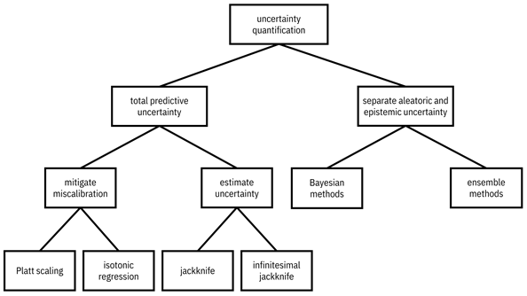
Figure 13.2. Different methods for quantifying the uncertainty of classifiers. Accessible caption. Hierarchy diagram with uncertainty quantification as the root. Uncertainty quantification has children total predictive uncertainty, and separate aleatoric and epistemic uncertainty. Total predictive uncertainty has children mitigate miscalibration and estimate uncertainty. Mitigate miscalibration has children Platt scaling and isotonic regression. Estimate uncertainty has children jackknife and infinitesimal jackknife. Separate aleatoric and epistemic uncertainty has children Bayesian methods and ensemble methods.
Just like in other pillars of trustworthiness, algorithms for obtaining uncertainty estimates and mitigating poor calibration apply at different stages of the machine learning pipeline. Unlike other topic areas, there is no pre-processing for uncertainty quantification. There are, however, methods that apply during model training and in post-processing. Two post-processing methods for mitigating poor calibration, Platt scaling and isotonic regression, both take the classifier’s existing calibration curve and straighten it out. Platt scaling assumes that the existing calibration curve looks like a sigmoid or logistic activation function whereas isotonic regression can work with any shape of the existing calibration curve. Isotonic regression requires more data than Platt scaling to work effectively.
A post-processing method for total predictive uncertainty quantification that does not require you to start with an existing classifier score works in almost the same way as computing deletion diagnostics described in Chapter 12 for explanation. You train many attrition models, leaving one training data point out each time. You compute the standard deviation of the accuracy of each of these models and report this number as an indication of predictive uncertainty. In the uncertainty quantification context, this is known as a jackknife estimate. You can do the same thing for other metrics of trustworthiness as well, yielding an extended table of results that goes beyond Table 13.1 to also contain uncertainty quantification, shown in Table 13.2. Such a table should be displayed in a factsheet.
Table 13.2. Result of testing several attrition models for multiple trust-related metrics with uncertainty quantified using standard deviation below the metric values.
|
Model |
Accuracy |
Accuracy with Distribution Shift |
Disparate Impact Ratio |
Empirical Robust-ness |
Faithful-ness |
|
logistic regression |
|
|
|
|
|
|
neural network |
|
|
|
|
|
|
decision forest (boosting) |
|
|
|
|
|
|
decision forest (bagging) |
|
|
|
|
|
Chapter 12 noted that deletion diagnostics are costly to compute directly, which motivated influence functions as an approximation for explanation. The same kind of approximation involving gradients and Hessians, known as an infinitesimal jackknife, can be done for uncertainty quantification.[19] Influence functions and infinitesimal jackknives may also be derived for some fairness, explainability, and robustness metrics.[20]
Using
a calibrated score or (infinitesimal) jackknife-based standard deviation as the
quantification of uncertainty does not allow you to decompose the total
predictive uncertainty into aleatoric and epistemic uncertainty, which can be
important as you decide to approve the JCN Corporation proactive retention
system. There are, however, algorithms applied during model training that let
you estimate the aleatoric and epistemic uncertainties separately. These
methods are like directly interpretable models (Chapter 12) and bias mitigation
in-processing (Chapter 10) in terms of their place in the pipeline. The basic
idea to extract the two uncertainties is as follows.[21]
The total uncertainty of a prediction, i.e. the predicted label ![]() given the features
given the features
![]() , is measured using
the entropy
, is measured using
the entropy ![]() (remember entropy
from Chapter 3). This prediction uncertainty includes both epistemic and
aleatoric uncertainty; it is general and does not fix the choice of the actual
classifier function
(remember entropy
from Chapter 3). This prediction uncertainty includes both epistemic and
aleatoric uncertainty; it is general and does not fix the choice of the actual
classifier function ![]() within a
hypothesis space
within a
hypothesis space ![]() . The epistemic
uncertainty component captures the lack of knowledge of a good hypothesis space
and a good classifier within a hypothesis space. Therefore, epistemic
uncertainty goes away once you fix the choice of hypothesis space and
classifier. All that remains is aleatoric uncertainty. The aleatoric uncertainty
is measured by another entropy
. The epistemic
uncertainty component captures the lack of knowledge of a good hypothesis space
and a good classifier within a hypothesis space. Therefore, epistemic
uncertainty goes away once you fix the choice of hypothesis space and
classifier. All that remains is aleatoric uncertainty. The aleatoric uncertainty
is measured by another entropy ![]() , averaged across classifiers
, averaged across classifiers
![]() whose probability
of being a good classifier is based on the training data. The epistemic
uncertainty is then the difference between
whose probability
of being a good classifier is based on the training data. The epistemic
uncertainty is then the difference between ![]() and the average
and the average ![]() .
.
There are a couple ways to obtain these two entropies and thereby the aleatoric and epistemic uncertainty. Bayesian methods, including Bayesian neural networks, are one large category of methods that learn full probability distributions for the features and labels, and thus the entropies can be computed from the probability distribution. The details of Bayesian methods are beyond the scope of this book.[22] Another way to obtain the aleatoric and epistemic uncertainty is through ensemble methods, including ones involving bagging and dropout that explicitly or implicitly create several independent machine learning models that are aggregated (bagging and dropout were described in Chapter 7).[23] The average classifier-specific entropy for characterizing aleatoric uncertainty is estimated by simply averaging the entropy of several data points for all the models in the trained ensemble considered separately. The total uncertainty is estimated by computing the entropy of the entire ensemble together.
13.3 Communicating Test Results and Uncertainty
Recall from Chapter 12, that you must overcome the cognitive biases of the consumer of an explanation. The same is true for communicating test results and uncertainty. Researchers have found that the presentation style has a large impact on the consumer.[24] So don’t take the shortcut of thinking that your job is done once you’ve completed the testing and uncertainty quantification. You’ll have to justify your model validation to several different factsheet consumers (internal stakeholders within JCN Corporation, external regulators, et al.) and it is important for you to think about how you’ll communicate the results.
13.3.1 Visualizing Test Results
Although tables of numbers such as Table 13.2 are complete and effective ways of conveying test results with uncertainty, there are some other options to consider. First, there are nascent efforts to use methods from explainability like contrastive explanations and influence functions to help consumers understand why a model has a given fairness metric or uncertainty level.[25] More importantly, visualization is a common approach.
The various trust dimension metrics you have tested are often presented as bar graphs. The trust metrics of multiple models can be compared with adjacent bars as in Figure 13.3. However, it is not clear whether this visualization is more effective than simply presenting a table like Table 13.1. Specifically, since model comparisons are to be done across dimensions that are on different scales, one dimension with a large dynamic range can warp the consumer’s perception. Also, if some metrics have better values when they are larger (e.g. accuracy) and other metrics have better values when they are smaller (e.g. statistical parity difference), the consumer can get confused when making comparisons. Moreover, it is difficult to see what is going on when there are several models (several bars).
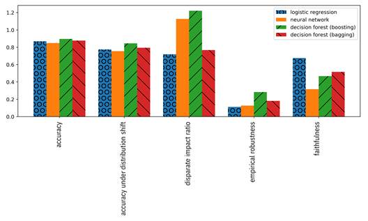
Figure 13.3. Bar graph of trust metrics for four different models.
An alternative is the parallel coordinate plot, which is a line graph of the different metric dimensions next to each other, but normalized separately.[26] An example is shown in Figure 13.4. The separate normalization per metric permits you to flip the direction of the axis so that, for example, higher is always better. (This flipping has been done for empirical robustness in the figure.) Since the lines can overlap, there is less of a crowding effect from too many models being compared than with bar graphs. (If there are so so many models that even the parallel coordinate plot becomes unreadable, an alternative is the parallel coordinate density plot, which gives an indication of how many lines there are in every part of the plot using shading.) The main purpose of parallel coordinate plots is precisely to compare items along several categories with different metrics. Conditional parallel coordinate plots, an interactive version of parallel coordinate plots, allow you to expand upon submetrics within a higher-level metric.[27] For example, if you create an aggregate metric that combines several adversarial robustness metrics including empirical robustness, CLEVER score, and others, an initial visualization will only contain the aggregate robustness score, but can be expanded to show the details of the other metrics it is composed of. Parallel coordinate plots can be wrapped around a polygon to yield a radar chart, an example of which is shown in Figure 13.5.
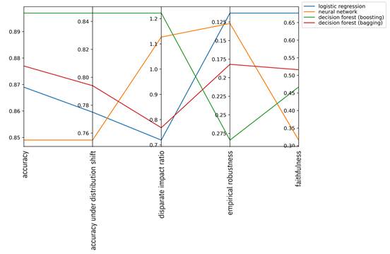
Figure 13.4. Parallel coordinate plot of trust metrics for four different models.
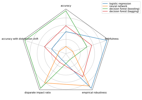
Figure 13.5. Radar chart of trust metrics for four different models.
It is not easy to visualize metrics such as disparate impact ratio in which both small and large values indicate poor performance and intermediate values indicate good values. In these cases, and also to appeal to less technical consumers in the case of all metrics, simpler non-numerical visualizations involving color patches (e.g. green/yellow/red that indicate good/medium/poor performance), pictograms (e.g. smiley faces or stars), or Harvey balls (○/◔/◑/◕/●) may be used instead. See Figure 13.6 for an example. However, these visualizations require thresholds to be set in advance on what constitutes a good, medium, or poor value. Eliciting these thresholds is part of value alignment, covered in Chapter 14.
|
Model |
Accuracy |
Accuracy with Distribution Shift |
Disparate Impact Ratio |
Empirical Robust-ness |
Faithful-ness |
|
logistic regression |
«««« |
«««« |
« |
««««« |
««««« |
|
neural network |
«««« |
«««« |
««« |
«««« |
« |
|
decision forest (boosting) |
««««« |
««««« |
« |
« |
««« |
|
decision forest (bagging) |
«««« |
«««« |
«« |
««« |
««« |
Figure 13.6. Simpler non-numeric visualization of trust metrics for four different models.
13.3.2 Communicating Uncertainty
It is critical that you not only present the test result facts in a meaningful way, but also present the uncertainty around those test results to ensure that employees receiving and not receiving retention incentives, their managers, other JCN Corporation stakeholders and external regulators have full transparency about the proactive retention system.[28] Van der Bles et al. give nine levels of communicating uncertainty:[29]
1. explicit denial that uncertainty exists,
2. no mention of uncertainty,
3. informally mentioning the existence of uncertainty,
4. a list of possibilities or scenarios,
5. a qualifying verbal statement,
6. a predefined categorization of uncertainty,
7. a rounded number, range or an order-of-magnitude assessment,
8. a summary of a distribution, and
9. a full explicit probability distribution.
You should not consider the first five of these options.
Similar to the green/yellow/red categories described above for test values, predefined categorizations of uncertainty, such as ‘extremely uncertain,’ ‘uncertain,’ ‘certain,’ and ‘extremely certain’ may be useful for less technical consumers. In contrast to green/yellow/red, categories of uncertainty need not be elicited during value alignment because they are more universal concepts that are not related to the actual metrics or use case. Ranges express the possibility function (presented in Chapter 3), and can also be useful presentations for less technical consumers.
The last two options are more appropriate for in-depth communication of uncertainty to consumers. Summaries of probability distributions, like the standard deviations given in Table 13.2, can also be shown in bar graphs using error bars. Box-and-whisker plots are like bar graphs, but show not only the standard deviation, but also outliers, quantiles and other summaries of uncertainty through a combination of marks, lines, and shaded areas. Violin plots are also like bar graphs, but show the full explicit probability distribution through their shape; the shape of the bar follows the pdf of the metric turned on its side. Examples of each are shown in Figure 13.7, Figure 13.8, and Figure 13.9. Parallel coordinate plots and radar charts can also contain error bars or shading to indicate summaries of probability distributions, but may be difficult to interpret when showing more than two or three models.
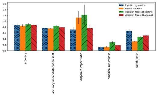
Figure 13.7. Bar graph with error bars of trust metrics for four different models.
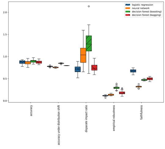
Figure 13.8. Box-and-whisker plot of trust metrics for four different models.
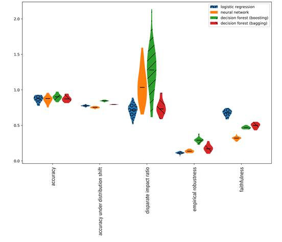
Figure 13.9. Violin plot of trust metrics for four different models.
13.4 Maintaining Provenance
In principle, factsheets are a good idea to achieve transparency, show conformity to regulations, and increase trustworthiness in JCN Corporation’s proactive retention system. But if consumers of factsheets think JCN Corporation is lying to them, is there anything you can do to convince them otherwise (assuming all the facts are impeccable)? More subtly, how can you show that facts haven’t been tampered with or altered after they were generated? Providing such assurance is hard because the facts are generated by many different people and processes throughout the development lifecycle, and just one weak link can spoil the entire factsheet. Provenance of the facts is needed.
One solution is a version of the fact flow tool with an immutable ledger as its storage back-end. An immutable ledger is a system of record whose entries (ideally) cannot be changed, so all facts are posted with a time stamp in a way that is very difficult to tamper. It is append-only, so you can only write to it and not change or remove any information. A class of technologies that implements immutable ledgers is blockchain networks, which use a set of computers distributed across many owners and geographies to each provably validate and store a copy of the facts. The only way to beat this setup is by colluding with more than half of the computer owners to change a fact that has been written, which is a difficult endeavor. Blockchains provide a form of distributed trust.
There are two kinds of blockchains: (1) permissioned (also known as private) and (2) permissionless (also known as public). Permissioned blockchains restrict reading and writing of information and ownership of machines to only those who have signed up with credentials. Permissionless blockchains are open to anyone and can be accessed anonymously. Either may be an option for maintaining the provenance of facts while making the attrition prediction model more trustworthy. If all consumers are within the corporation or are among a fixed set of regulators, then a permissioned blockchain network will do the trick. If the general public or others external to JCN Corporation are the consumers of the factsheet, then a permissionless blockchain is the preferred solution.
Posting facts to a blockchain solves the problem of maintaining the provenance of facts, but what if there is tampering in the creation of the facts themselves? For example, what if a data scientist discovers a small bug in the feature engineering code that shouldn’t affect model performance very much and fixes it. Retraining the entire model will go on through the night, but there’s a close-of-business deadline to submit facts. So the data scientist submits facts from a previously trained model. Shortcuts like this can also be prevented with blockchain technologies.[30] Since the training of many machine learning models is done in a deterministic way by an iterative procedure (such as gradient descent), other computers in the blockchain network can endorse and verify that the training computation was actually run by locally rerunning small parts of the computation starting from checkpoints of the iterations posted by the data scientist. The details of how to make such a procedure tractable in terms of computation and communication costs is beyond the scope of the book.
In your testing, you found that all of the models were lacking in fairness, so you sent them back to the data scientists to add better bias mitigation, which they did to your satisfaction. The various stakeholders are satisfied now as well, so you can go ahead and sign for the system’s conformity and push it on to the deployment stage of the lifecycle. Alongside the deployment efforts, you also release a factsheet for consumption by the managers within JCN Corporation who will be following through on the machine’s recommended retention actions. Remember that one of the promises of this new machine learning system was to make employment at JCN Corporation more equitable, but that will only happen if the managers adopt the system’s recommendations.[31] Your efforts at factsheet-based transparency have built enough trust among the managers so they are willing to adopt the system, and JCN Corporation will have fairer decisions in retention actions.
13.5 Summary
§ Transparency is a key means for increasing the third attribute of trustworthiness in machine learning (openness and human interaction).
§ Fact flow is a mechanism for automatically collecting qualitative and quantitative facts about a development lifecycle. A factsheet is a collection of facts, appropriately rendered for a given consumer, that enables transparency and conformity assessment.
§ Model validation and risk management involve testing models across dimensions of trust, computing the uncertainties of the test results, capturing qualitative facts about the development lifecycle, and documenting and communicating these items transparently via factsheets.
§ Testing machine learning models is a unique endeavor different from other software testing because of the oracle problem: not knowing in advance what the behavior should be.
§ Visualization helps make test results and their uncertainties more accessible to various consumer personas.
§ Facts and factsheets become more trustworthy if their provenance can be maintained and verified. Immutable ledgers implemented using blockchain networks provide such capabilities.