1       

2       

3       

4       

5       

6       

7       

8       

9       

10       

11       

12       

Interpretability and Explainability

Hilo is a (fictional) startup company trying to shake up the online second home mortgage market. A type of second mortgage known as a home equity line of credit (HELOC) allows customers to borrow intermittently using their house as collateral. Hilo is creating several unique propositions to differentiate itself from other companies in the space. The first is that it integrates the different functions involved in executing a second mortgage, including a credit check of the borrower and an appraisal of the value of the home, in one system. Second, its use of machine learning throughout these human decision-making processes is coupled with a maniacal focus on robustness to distribution shift, fairness, and adversarial robustness. Third, it has promised to be scrutable to anyone who would like to examine the machine learning models it will use and to provide avenues for recourse if the machine’s decisions are problematic in any respect. Imagine that you are on the data science team assembled by Hilo and have been tasked with addressing the third proposition by making the machine learning models interpretable and explainable. The platform’s launch date is only a few months away, so you had better get cracking.

Interpretability of machine learning models is the aim to let people understand how the machine makes its predictions. It is a challenge because many of the machine learning approaches in Chapter 7 are not easy for people to understand since they have complicated functional forms. Interpretability and explainability are a form of interaction between the machine and a human, specifically communication from the machine to the human, that allow the machine and human to collaborate in decision making.[1] This topic and chapter lead off Part 5 of the book on interaction, which is the third attribute of trustworthiness of machine learning. Remember that the organization of the book matches the attributes of trustworthiness, shown in Figure 12.1.

 

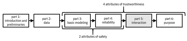
Figure 12.1. Organization of the book. The fifth part focuses on the third attribute of trustworthiness, intimacy or interaction, which maps to machine learning models that can communicate with people and receive instruction from people about their values. Accessible caption. A flow diagram from left to right with six boxes: part 1: introduction and preliminaries; part 2: data; part 3: basic modeling; part 4: reliability; part 5: interaction; part 6: purpose. Part 5 is highlighted. Parts 3–4 are labeled as attributes of safety. Parts 3–6 are labeled as attributes of trustworthiness.

The typical output of a machine learning model is the predicted label , but this label is not enough to communicate how the machine makes its predictions. Something more, in the form of an explanation, is also needed. The machine is the transmitter of information and the human is the receiver or consumer of that information. As shown in Figure 12.2, the communication process has to overcome human cognitive biases—the limitations that people have in receiving information—that threaten human-machine collaboration. This is sometimes known as the last mile problem.[2] The figure completes the picture of biases and validities you’ve seen starting in Chapter 4. The final space is the perceived space, which is the final understanding that the human consumer has of the predictions from Hilo’s machine learning models.

You will not be able to create a single kind of explanation that appeals to all of the different potential consumers of explanations for Hilo’s models. Even though the launch date is only a few months away, don’t take the shortcut of assuming that any old explanation will do. The cognitive biases of different people are different based on their persona, background, and purpose. As part of the problem specification phase of the machine learning lifecycle, you’ll first have to consider all the different types of explanations at your disposal before going into more depth on any of them during the modeling phase.

 

12.1       The Different Types of Explanations

Just like we as people have many ways to explain things to each other, there are many ways for machine learning models to explain their predictions to consumers. As you consider which ones you’ll need for Hilo’s models, you should start by enumerating the personas of consumers.

 

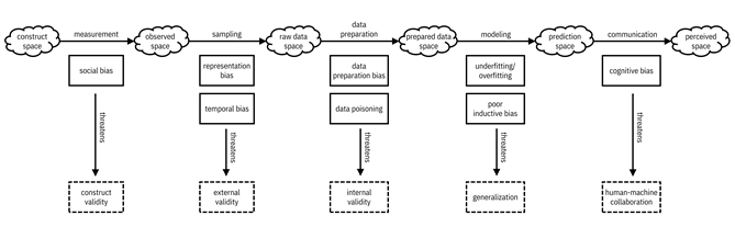
Figure 12.2. A mental model of spaces, validities, and biases. The final space is the perceived space, which is what the human understands from the machine’s output. Accessible caption. A sequence of six spaces, each represented as a cloud. The construct space leads to the observed space via the measurement process. The observed space leads to the raw data space via the sampling process. The raw data space leads to the prepared data space via the data preparation process. The prepared data space leads to the prediction space via the modeling process. The prediction space leads to the perceived space via the communication process. The measurement process contains social bias, which threatens construct validity. The sampling process contains representation bias and temporal bias, which threatens external validity. The data preparation process contains data preparation bias and data poisoning, which threaten internal validity. The modeling process contains underfitting/overfitting and poor inductive bias, which threaten generalization. The communication process contains cognitive bias, which threatens human-machine collaboration.

12.1.1     Personas of the Consumers of Explanations

The first consumer is the decision maker who collaborates with the machine learning system to make the prediction: the appraiser or credit officer. These consumers need to understand and trust the model and have enough information about machine predictions to combine with their own inclinations to produce the final decision. The second consumer persona is the HELOC applicant. This affected user would like to know the factors that led to their model-predicted home appraisal and creditworthiness, and what they can do to improve these predictions. The third main persona of consumers is an internal compliance official or model validator, or an official from an external regulatory agency that ensures that the decisions are not crossing any legal boundaries. Together, all of these roles are regulators of some sort. The fourth possible consumer of explanations is a data scientist in your own team at Hilo. Explanations of the functioning of the models can help a member of your team debug and improve the models.

“If we don’t know what is happening in the black box, we can’t fix its mistakes to make a better model and a better world.”

—Aparna Dhinakaran, chief product officer at Arize AI

Note that unlike the other three personas, the primary concern of the data scientist persona is not building interaction and intimacy for trustworthiness. The four different personas and their goals are summarized in Table 12.1.

Table 12.1. The four main personas of consumers of explanations and their goals.

Persona	Example	Goal
decision maker	appraiser, credit officer	(1) roughly understand the model to gain trust; (2) understand the predictions to combine with their own information to make decisions
affected user	HELOC applicant	understand the prediction for their own input data point and what they can do to change the outcome
regulator	model validator, government official	ensure the model is safe and compliant
data scientist	Hilo team member	improve the model’s performance

 

12.1.2     Dichotomies of Explanation Methods

To meet the goals of the different personas, one kind of explanation is not enough.[3] You’ll need several different explanation types for Hilo’s systems. There are three dichotomies that delineate the methods and techniques for machine learning explainability.

§  The first dichotomy is local vs. global: is the consumer interested in understanding the machine predictions for individual input data points or in understanding the model overall.

§  The second dichotomy is exact vs. approximate: should the explanation be completely faithful to the underlying model or is some level of approximation allowable.

§  The third dichotomy is feature-based vs. sample-based: is the explanation given as a statement about the features or is it given by pointing to other data points in their entirety. Feature-based explanations require that the underlying features be meaningful and understandable by the consumer. If they are not already meaningful, a pre-processing step known as disentangled representation may be required. This pre-processing finds directions of variation in semi-structured data that are not necessarily aligned to the given features but have some human interpretation, and is expanded upon in Section 12.2.

Since there are three dichotomies, there are eight possible combinations of explanation types. Certain types of explanations are more appropriate for certain personas to meet their goals. The fourth persona, data scientists from your own team at Hilo, may need to use any and all of the types of explanations to debug and improve the model.

§  Local, exact, feature-based explanations help affected users such as HELOC applicants gain recourse and understand precisely which feature values they have to change in order to pass the credit check.

§  Global and local approximate explanations help decision makers such as appraisers and credit officers achieve their dual goals of roughly understanding how the overall model works to develop trust in it (global) and having enough information about a machine-predicted property value to combine with their own information to produce a final appraisal (local).

§  Global and local, exact, sample-based explanations and global, exact, feature-based explanations help regulators understand the behavior and predictions of the model as a safeguard. By being exact, the explanations apply to all data points, including edge cases that might be washed out in approximate explanations. Of these, the local, exact, sample-based and global, exact, feature-based explanations that appeal to regulators come from directly interpretable models.

§  Regulators and decision makers can both benefit from global, approximate, sample-based explanations to gain understanding.

The mapping of explanation types to personas is summarized in Table 12.2.

Table 12.2. The three dichotomies of explanations and their mapping to personas.

Dichotomy 1	Dichotomy 2	Dichotomy 3	Persona	Example Method
local	exact	feature-based	affected user	contrastive explanations method
local	exact	sample-based	regulator	k-nearest neighbor
local	approximate	feature-based	decision maker	LIME, SHAP, saliency map
local	approximate	sample-based	decision maker	prototype
global	exact	feature-based	regulator	decision tree, Boolean rule set, logistic regression, GAM, GLRM
global	exact	sample-based	regulator	deletion diagnostics
global	approximate	feature-based	decision maker	distillation, SRatio, partial dependence plot
global	approximate	sample-based	regulator and decision maker	influence function

 

Another dichotomy that you might consider in the problem specification phase is whether you will allow the explanation consumer to interactively probe the Hilo machine learning system to gain further insight, or whether the system will simply produce static output explanations that the consumer cannot further interact with. The interaction can be through natural language dialogue between the consumer and the machine, or it could be by means of visualizations that the consumer adjusts and drills down into.[4] The variety of static explanations is already plenty for you to deal with without delving into interaction, so you decide to proceed only with static methods.

 Mirroring the three points of intervention in the modeling pipeline seen in Part 4 of the book for distributional robustness, fairness, and adversarial robustness, Figure 12.3 shows different actions for interpretability and explainability. As mentioned earlier, disentangled representation is a pre-processing step. Directly interpretable models arise from training decision functions in specific constrained hypothesis classes (recall that the concept of hypothesis classes was introduced in Chapter 7). Finally, many methods of explanation are applied on top of already-trained, non-interpretable models such as neural networks in a post hoc manner.

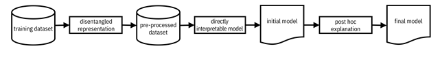
Figure 12.3. Pipeline view of explanation methods. Accessible caption. A block diagram with a training dataset as input to a disentangled representation block with a pre-processed dataset as output. The pre-processed dataset is input to a directly interpretable model block with an initial model as output. The initial model is input to a post hoc explanation block with a final model as output.

12.1.3     Conclusion

Now you have the big picture view of different explanation methods, how they help consumers meet their goals, and how they fit into the machine learning pipeline steps. The appraisal and HELOC approval systems you’re developing for Hilo require you to appeal to all of the different consumer types, and you have the ability to intervene on all parts of the pipeline, so you should start putting together a comprehensive toolkit of interpretable and explainable machine learning techniques.

 

12.2       Disentangled Representation

Before people can start understanding how models make their predictions, they need some understanding of the underlying data. Features in tabular and other structured data used as inputs to machine learning models can usually be understood by consumers in some capacity. Consumers who are not decision makers, regulators, or other domain experts (or even if they are) might not grasp the nuance of every feature, but they can at least consult a data dictionary to get some understanding of each one. For example, in the HELOC approval model, a feature ‘months since most recent delinquency’ might not make total sense to applicants, but it is something they can understand if they do some research about it.

The same is not true of semi-structured data. For example, inputs to the home appraisal model include satellite and street view images of the property and surrounding neighborhood. The features are individual red, blue, and green color values for each pixel of the image. Those features are not meaningful to any consumer. They are void of semantics. Higher-level representations, for example edges and textures that are automatically learned by neural networks, are a little better but still leave an explanation consumer wanting. They do not directly have a meaning in the context of a home appraisal.

What can be done instead? The answer is a representation in which the dimensions are the amount of foliage in the neighborhood, the amount of empty street frontage, the visual desirability of the house, etc.[5] that are uncorrelated with each other and also provide information not captured in other input data. (For example, even though the size and number of floors of the home could be estimated from images, it will already be captured in other tabular data.) Such a representation is known as a disentangled representation. The word disentangled is used because in such a representation, intervening on one dimension does not cause other dimensions to also change. Recently developed methods can learn disentangled representations directly from unlabeled data.[6] Although usually not the direct objective of disentangling, such representations tend to yield meaningful dimensions that people can provide semantics to, such as the example of ‘foliage in the neighborhood’ mentioned above. Therefore, disentangled representation is a way of pre-processing the training data features to make them more human-interpretable. Modeling and explanation methods later in the pipeline take the new features as input.

Sometimes, disentangled representation to improve the features is not good enough to provide meaning to consumers. Similarly, sometimes tabular data features are just not sufficient to provide meaning to a consumer. In these cases, an alternative pre-processing step is to directly elicit meaningful explanations from consumers, append them to the dataset as an expanded cardinality label set, and train a model to predict both the original appraisal or creditworthiness as well as the explanation.[7]

 

12.3       Explanations for Regulators

Directly interpretable models are simple enough for consumers to be able to understand exactly how they work by glancing at their form. They are appropriate for regulators aiming for model safety. They are a way to reduce epistemic uncertainty and achieve inherently safe design: models that do not have any spurious components.[8] The explanation is done by restricting the hypothesis class from which the decision function is drawn to only those functions that are simple and understandable. There are two varieties of directly interpretable exact models: (1) local sample-based and (2) global feature-based. Moreover, model understanding by regulators is enhanced by global sample-based explanations, both exact and approximate.

12.3.1     k-Nearest Neighbor Classifier

The k-nearest neighbor classifier introduced in Chapter 7 is the main example of a local sample-based directly interpretable model. The predicted creditworthiness or appraisal label is computed as the average label of nearby training data points. Thus, a local explanation for a given input data point is just the list of the k-nearest neighbor samples, including their labels. This list is simple enough for regulators to understand. You can also provide the distance metric for additional understanding.

12.3.2     Decision Trees and Boolean Rule Sets

There is more variety in global feature-based directly interpretable models. Decision trees, introduced in Chapter 7, can be understood by regulators by tracing paths from the root through intermediate nodes to leaves containing predicted labels.[9] The individual features and thresholds involved in each node are explicit and well-understood. A hypothesis class similar to decision trees is Boolean rule sets (OR-of-AND rules and AND-of-OR rules) that people are able to comprehend directly. They are combinations of decision stumps or one-rules introduced in Chapter 7. An example of an OR-of-AND rule classifier for HELOC creditworthiness is one that predicts the applicant to be non-creditworthy if:[10]

§  (Number of Satisfactory Trades ≤ 17 AND External Risk Estimate ≤ 75) OR

§  (Number of Satisfactory Trades > 17 AND External Risk Estimate ≤ 72).

This is a very compact rule set in which regulators can easily see the features involved and their thresholds. They can reason that the model is more lenient on external risk when the number of satisfactory trades is higher. They can also reason that the model does not include any objectionable features. (Once decision trees or Boolean rule sets become too large, they start becoming less interpretable.)

One common refrain that you might hear is of a tradeoff between accuracy and interpretability. This argument is false.[11] Due to the Rashomon effect introduced in Chapter 9, many kinds of models, including decision trees and rule sets, have almost equally high accuracy on many datasets. The domain of competence for decision trees and rule sets is broad (recall that the domain of competence introduced in Chapter 7 is the set of dataset characteristics on which a type of model performs well compared to other models). While it is true that scalably training these models has traditionally been challenging due to their discrete nature (discrete optimization is typically more difficult than continuous optimization), the challenges have recently been overcome.[12]

“Simplicity is not so simple.”

—Dmitry Malioutov, computer scientist at IBM Research

When trained using advanced discrete optimization, decision trees and Boolean rule set classifiers show competitive accuracies across many datasets.

12.3.3     Logistic Regression

Linear logistic regression is also considered by many regulators to be directly interpretable. Recall from Chapter 7 that the form of the linear logistic regression decision function is . The -dimensional weight vector  has one weight per feature dimension in , which are different attributes of the HELOC applicant. These weight and feature dimensions are and , respectively, which get multiplied and summed as:  before going into the step function. In logistic regression, the relationship between the probability  (also the score ) and the weighted sum of feature dimensions is:

Equation 12.1

which you’ve seen before as the logistic activation function for neural networks in Chapter 7. It can be rearranged to the following:

Equation 12.2

The left side of Equation 12.2 is called the log-odds. When the log-odds is positive,  is the more likely prediction: creditworthy. When the log-odds is negative,  is the more likely prediction: non-creditworthy.

The way to understand the behavior of the classifier is by examining how the probability, the score, or the log-odds change when you increase an individual feature attribute’s value by . Examining the response to changes is a general strategy for explanation that recurs throughout the chapter. In the case of linear logistic regression, an increase of feature value by  while leaving all other feature values constant adds  to the log-odds. The weight value has a clear effect on the score. The most important features per unit change of feature values are those with the largest absolute values of the weights. To more easily compare feature importance using the weights, you should first standardize each of the features to zero mean and unit standard deviation. (Remember that standardization was first introduced when evaluating the covariate balancing of causal models in Chapter 8.)

12.3.4     Generalized Additive Models

Generalized additive models (GAMs) are a class of models that extend linear logistic regression to be nonlinear while retaining the same approach for interpretation. Instead of scalar weights multiplying feature values in the decision function for credit check prediction: , nonlinear functions are applied: . The entire function for a given feature dimension explicitly adds to the log-odds or subtracts from it. You can only do this exactly because there is no interaction between the feature dimensions. You can choose any hypothesis class for the nonlinear functions, but be aware that the learning algorithm has to fit the parameters of the functions from training data. Usually, smooth spline functions are chosen. (A spline is a function made up of piecewise polynomials strung together.)

12.3.5     Generalized Linear Rule Models

What if you want the regulators to have an easy time understanding the nonlinear functions involved in the HELOC decision function themselves? You can choose the nonlinear functions to be Boolean one-rules or decision stumps involving single features. The generalized linear rule model (GLRM) is exactly what you need: a directly interpretable method that combines the best of Boolean rule sets and GAMs.[13] In addition to Boolean one-rules of feature dimensions, the GLRM can have plain feature dimensions too. An example GLRM for HELOC credit checks is shown in Table 12.3.

Table 12.3. An example generalized linear rule model for HELOC credit checks.

Plain Feature or First-Degree Boolean Rule	Weight
Months Since Most Recent Inquiry[14] > 0
Months Since Most Recent Inquiry = 0
(Standardized) External Risk Estimate
External Risk Estimate > 75
External Risk Estimate > 72
External Risk Estimate > 69
(Standardized) Revolving Balance Divided by Credit Limit
Revolving Balance Divided by Credit Limit ≤ 39
Revolving Balance Divided by Credit Limit ≤ 50
(Standardized) Number of Satisfactory Trades
Number of Satisfactory Trades ≤ 12
Number of Satisfactory Trades ≤ 17

 

The three plain features (‘external risk estimate’, ‘revolving balance divided by credit limit’, and ‘number of satisfactory trades’) were standardized before doing anything else, so you can compare the weight values to see which features are important. The decision stump of ‘months since most recent inquiry’ being greater than zero is the most important because it has the largest coefficient. The decision stump of ‘external risk estimate’ being greater than 69 is the least important because it has the smallest coefficient. This is the same kind of understanding that you would apply to a linear logistic regression model.

The way to further understand this model is by remembering that the weight contributes to the log-odds for every unit change of the feature. Taking the ‘external risk estimate’ feature as an example, the GLRM tells you that:

§      for every increase of External Risk Estimate by , increase the log-odds by  (this number is obtained by undoing the standardization on the weight );

§      if External Risk Estimate > 69, increase log-odds by an additional ;

§      if External Risk Estimate > 72, increase log-odds by an additional ;

§      if External Risk Estimate > 75, increase log-odds by an additional .

The rule is fairly straightforward for consumers such as regulators to understand while being an expressive model for generalization. As shown in Figure 12.4, you can plot the contributions of the ‘external risk estimate’ feature to the log-odds to visually see how the Hilo classifier depends on it. Plots of  for other GAMs look similar, but can be nonlinear in different ways.

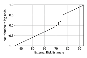
Figure 12.4. Contribution of the ‘external risk estimate’ feature to the log-odds of the classifier. Accessible caption. A plot with contribution to log-odds on the vertical axis and external risk estimate on the horizontal axis. The contribution to log-odds function increases linearly with three jump discontinuities.

You can also ‘undo’ the log-odds to get the actual probability (Equation 12.1 instead of Equation 12.2), but it is not additive like the log-odds. Nevertheless, the shape of the probability curve is informative in the same way, and is shown in Figure 12.5.

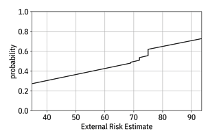
Figure 12.5. Contribution of the ‘external risk estimate’ feature to the probability of the classifier. Accessible caption. A plot with probability on the vertical axis and external risk estimate on the horizontal axis. The probability function increases linearly with three jump discontinuities.

GA²Ms, equivalently known as explainable boosting machines, are directly interpretable models that work the same as GAMs, but with two-dimensional nonlinear interaction terms .[15] Visually showing their contribution to the log-odds of the classifier requires two-dimensional plots. It is generally difficult for people to understand interactions involving more than two dimensions and therefore higher-order GA²Ms are not used in practice.[16] However, if you allow higher-degree rules in GLRMs, you end up with GA²Ms of AND-rules or OR-rules involving multiple interacting feature dimensions that unlike general higher-order GA²Ms, are still directly interpretable because rules involving many features can be understood by consumers.

12.3.6     Deletion Diagnostics and Influence Functions

The final set of methods that appeal to the regulator persona are from the global sample-based category. An exact method computes deletion diagnostics to find influential instances and an approximate method uses influence functions to do the same. The basic idea of deletion diagnostics is simple. You train a model with the entire training dataset of houses or applicants and then train it again leaving out one of the training samples. Whatever global changes there are to the model can be attributed to the house or applicant that you left out. How do you look at what changed between the two models? You can directly look at the two models or their parameters, which makes sense if the models are interpretable. But that won’t work if you have an uninterpretable model. What you need to do is evaluate the two models on a held-out test set and compute the average change in the predicted labels. The bigger the change, the more influential the training data point. The regulator gains an understanding of the model by being given a list of the most influential homes or applicants.

Exactly computing deletion diagnostics is expensive because you have to train  different models, leaving one training point out each time plus the model trained on all the data points. So usually, you’ll want to approximate the calculation of the most influential training samples. Let’s see how this approximation is done for machine learning algorithms that have smooth loss functions using the method of influence functions (refer back to Chapter 7 for an introduction to loss functions).[17] Influence function explanations are also useful for decision makers.

The method for computing the influence of a certain training data point  on a held-out test data point  starts by approximating the loss function by quadratic functions around each training data point. The gradient vector  (slope or set of first partial derivatives) and Hessian matrix  (local curvature or set of second partial derivatives) of the quadratic approximations to the loss function with respect to the model’s parameters are then calculated as closed-form formulas. The average of the Hessian matrices across all the training data points is also computed and denoted by . Then the influence of sample  on  is .

The expression takes this form because of the following reason. First, the  part of the expression is a step in the direction toward the minimum of the loss function at  (for those who have heard about it before, this is the Newton direction). Taking a step toward the minimum affects the model parameters just like deleting  from the training dataset, which is what the deletion diagnostics method does explicitly. The expression involves both the slope and the local curvature because the steepest direction indicated by the slope is bent towards the minimum of quadratic functions by the Hessian. Second, the  part of the expression maps the overall influence of  to the  sample. Once you have all the influence values for a set of held-out test houses or applicants, you can average, rank, and present them to the regulator to gain global understanding about the model.

 

12.4       Explanations for Decision Makers

Decision trees, Boolean rule sets, logistic regression, GAMs, GLRMs, and other similar hypothesis classes are directly interpretable through their features because of their relatively simple form. However, there are many instances in which you want to or have to use a complicated uninterpretable model. (Examples of uninterpretable models include deep neural networks as well as decision forests and other similar ensembles that you learned in Chapter 7.) Nevertheless, in these instances, you want the decision maker persona to have a model-level global understanding of how the Hilo model works. What are the ways in which you can create approximate global explanations to meet this need? (Approximation is a must. If a consumer could understand the complicated model without approximation, it would be directly interpretable already.) There are two ways to approach global approximate feature-based explanations: (1) training a directly interpretable model like a decision tree, rule set, or GAM to be similar to the uninterpretable model, or (2) computing global summaries of the uninterpretable model that are understandable. In both cases, you first fit the complicated uninterpretable model using the training data set.

In addition to having a general model-level understanding to develop trust, approximate explanations at the local level help the appraiser or credit officer understand the predictions to combine with their own information to make decisions. The local feature-based explanation methods LIME and SHAP extend each of the two global feature-based explanation methods to the local level, respectively. A third local feature-based explanation method useful to appraisers and usually applied to semi-structured data modalities is known as saliency maps. Finally, local approximate sample-based explanations based on comparisons to prototypical data points help appraisers and credit officers make their final decisions as well. All of these methods are elaborated upon in this section.

12.4.1     Global Model Approximation

Global model approximation is the idea of finding a directly interpretable model that is close to a complicated uninterpretable model. It has two sub-approaches. The first, known as distillation, changes the learning objective of the directly interpretable model from the standard risk minimization objective to an objective of matching the uninterpretable model as closely as possible.[18]

The second sub-approach for approximation using directly interpretable models, known as SRatio, computes training data weights based on the uninterpretable model and interpretable model. Then it trains the directly interpretable model with the instance weights.[19] You’ve seen reweighing of data points repeatedly in the book: inverse probability weighting for causal inference, confusion matrix-based weights to adapt to prior probability shift, importance weights to adapt to covariate shift, and reweighing as a pre-processing bias mitigation algorithm. The general idea here is the same, and is almost a reversal of importance weights for covariate shift.

Remember from Chapter 9 that in covariate shift settings, the training and deployment feature distributions are different, but the labels given the features are the same:  and . The importance weights are then: . For explanation, there is no separate training and deployment distribution; there is an uninterpretable and an interpretable model. Also, since you’re explaining the prediction process, not the data generating process, you care about the predicted label  instead of the true label . The feature distributions are the same because you train the uninterpretable and interpretable models on the same training data houses or applicants, but the predicted labels given the features are different since you’re using different models:  and .

So following the same pattern as adapting to covariate shift by computing the ratio of the probabilities that are different, the weights are: . You want the interpretable model to look like the uninterpretable model. In the weight expression, the numerator comes from the classifier score of the trained uninterpretable model and the denominator comes from the score of the directly interpretable model trained without weights.

12.4.2     LIME

Global feature-based explanation using model approximation has an extension to the local explanation case known as local interpretable model-​agnostic explanations (LIME). The idea is similar to the global method from the previous subsection. First you train an uninterpretable model and then you approximate it by fitting a simple interpretable model to it. The difference is that you do this approximation around each deployment data point separately rather than trying to come up with one overall approximate model.

To do so, you get the uninterpretable model’s prediction on the deployment data point you care about, but you don’t stop there. You add a small amount of noise to the deployment data point’s features several times to create a slew of perturbed input samples and classify each one. You then use this new set of data points to train the directly interpretable model. The directly interpretable model is a local approximation because it is based only on a single deployment data point and a set of other data points created around it. The interpretable model can be a logistic regression or decision tree and is simply shown to the decision maker, the Hilo appraiser or credit officer.

12.4.3     Partial Dependence Plots

The second global approach for increasing the trust of the appraisers and credit officers is the approximate feature-based explanation method known as partial dependence plots. The main idea is simple: compute and plot the classifier probability as a function of each of the feature dimensions  separately, that is . You know exactly how to compute this partial dependence function from Chapter 3 by integrating or summing the probability  over all the feature dimensions except dimension , also known as marginalization. An example partial dependence plot for the ‘external risk estimate’ feature is shown in Figure 12.6.

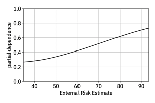
Figure 12.6. Partial dependence plot of the ‘external risk estimate’ feature for some uninterpretable classifier model. Accessible caption. A plot with partial dependence on the vertical axis and external risk estimate on the horizontal axis. The partial dependence smoothly increases in a sigmoid-like shape.

The plot of an individual feature’s exact contribution to the probability in Figure 12.5 for GAMs looks similar to a partial dependence plot in Figure 12.6 for an uninterpretable model, but is different for one important reason. The contributions of the individual features exactly combine to recreate a GAM because the different features are unlinked and do not interact with each other. In uninterpretable models, there can be strong correlations and interactions among input feature dimensions exploited by the model for generalization. By not visualizing the joint behaviors of multiple features in partial dependence plots, an understanding of those correlations is lost. The set of all  partial dependence functions is not a complete representation of the classifier. Together, they are only an approximation to the complete underlying behavior of the creditworthiness classifier.

12.4.4     SHAP

Just like LIME is a local version of global model approximation, a method known as SHAP is a local version of partial dependence plots. The partial dependence plot shows the entire curve of partial dependence across all feature values, whereas SHAP focuses on the precise point on the feature axis corresponding to a particular applicant in the deployment data. The SHAP value is simply the difference between the partial dependence value for that applicant and the average probability, shown in Figure 12.7.

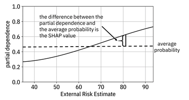
Figure 12.7. Example showing the SHAP value as the difference between the partial dependence and average probability for a given applicant’s ‘external risk estimate’ value. Accessible caption. A plot with partial dependence on the vertical axis and external risk estimate on the horizontal axis. The partial dependence smoothly increases in a sigmoid-like shape. A horizontal line passing through the partial dependence function marks the average probability. The difference between the partial dependence and the average probability is the SHAP value.

12.4.5     Saliency Maps

Another local explanation technique for you to consider adding to your Hilo explainability toolkit takes the partial derivative of the classifier’s score  or probability of label  with respect to each of the input feature dimensions , . A higher magnitude of the derivative indicates a greater change in the classifier score with a change in the feature dimension value, which is interpreted as greater importance of that feature. Putting together all  of the partial derivatives, you have the gradient of the score with respect to the features  that you examine to see which entries have the largest absolute values. For images, the gradient can be displayed as another image known as a saliency map. The decision maker can see which parts of the image are most important to the classification. Saliency map methods are approximate because they do not consider interactions among the different features.

Figure 12.8 shows example saliency maps for a classifier that helps the appraisal process by predicting what objects are seen in a street view image. The model is the Xception image classification model trained on the ImageNet Large Scale Visual Recognition Challenge dataset containing 1000 different classes of objects.[20] The saliency maps shown in the figure are computed by a specific method known as grad-CAM.[21] It is clear from the saliency maps that the classifier focuses its attention on the main house portion and its architectural details, which is to be expected.

  

  

Figure 12.8. Two examples of grad-CAM applied to an image classification model. The left column is the input image, the middle column is the grad-CAM saliency map with white indicating higher attribution, and the right column superimposes the attribution on top of the image. The top row image is classified by the model as a ‘mobile home’ and the bottom row image is classified as a ‘palace.’ (Both classifications are incorrect.) The salient architectural elements are correctly highlighted by the explanation algorithm in both cases. Accessible caption. In the first example, the highest attribution on a picture of a townhouse is on the windows, stairs, and roof. In the second example, the highest attribution on a picture of a colonial-style house is on the front portico.

12.4.6     Prototypes

Another kind of explanation useful for the decision maker persona, appraiser or credit officer, is through local sample-based approximations of uninterpretable models. Remember that local directly interpretable models, such as the k-nearest neighbor classifier work by averaging the labels of nearby HELOC applicant data points. The explanation is just the list of those other applicants and their labels. However, it is not required that a sample-based explanation only focus on nearby applicants. In this section, you will learn an approach for approximate local sample-based explanation that presents prototypical applicants as its explanation.

Prototypes—data points in the middle of a cluster of other data points shown in Figure 12.9—are useful ways for consumers to perform case-based reasoning to gain understanding of a classifier.[22] This reasoning is as follows. To understand the appraised value of a house, compare it to the most prototypical other house in the neighborhood that is average in every respect: average age, average square footage, average upkeep, etc. If the appraised value of the house in question is higher than the prototype, you can see which features have better values and thus get a sense of how the classifier works, and vice versa.

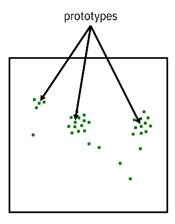
Figure 12.9. Example of a dataset with three prototype samples marked. Accessible caption. A plot with several data points, some of which are clustered into three main clusters. Central datapoints within those clusters are marked as prototypes.

However, just showing the one nearest prototype is usually not enough. You’ll also want to show a few other nearby prototypes so that the consumer can gain even more intuition. Importantly, listing several nearby prototypes to explain an uninterpretable model and listing several nearby data points to explain the k-nearest neighbor classifier is not the same. It is often the case that the several nearby house data points are all similar to each other and do not provide any further intuition than any one of them alone. With nearby prototype houses, each one is quite different from the others and therefore does provide new understanding.

Let’s look at examples of applicants in deployment data whose creditworthiness was predicted by an uninterpretable Hilo model along with three of their closest prototypes from the training data. As a first example, examine an applicant predicted to be creditworthy by the model. The labels of the prototypes must match that of the data point. The example creditworthy applicant’s prototype explanation is given in Table 12.4.

The data point and the nearest prototype are quite similar to each other, but with the applicant having a slightly lower ‘external risk estimate’ and slightly longer time since the oldest trade. It makes sense that the applicant would be predicted to be creditworthy just like the first prototype, even with those differences in ‘external risk estimate’ and ‘months since oldest trade open.’ The second nearest prototype represents applicants who have been in the system longer but have executed fewer trades, and have a lower ‘external risk estimate.’ The decision maker can understand from this that the model is willing to predict applicants as creditworthy with lower ‘external risk estimate’ values if they counteract that low value with longer time and fewer trades. The third nearest prototype represents applicants who have been in the system even longer, executed even fewer trades, have never been delinquent, and have a very high ‘external risk estimate’: the really solid applicants.

 

 

Table 12.4. An example prototype explanation for a HELOC applicant predicted to be creditworthy.

Feature	Applicant (Credit-worthy)	Nearest Prototype	Second Prototype	Third Prototype
External Risk Estimate	82	85	77	89
Months Since Oldest Trade Open	280	223	338	379
Months Since Most Recent Trade Open	13	13	2	156
Average Months in File	102	87	109	257
Number of Satisfactory Trades	22	23	16	3
Percent Trades Never Delinquent	91	91	90	100
Months Since Most Recent Delinquency	26	26	65	0
Number of Total Trades	23	26	21	3
Number of Trades Open in Last 12 Months	0	0	1	0
Percent Installment Trades	9	9	14	33
Months Since Most Recent Inquiry	0	1	0	0
Revolving Balance Divided by Credit Limit	3	4	2	0

 

As a second example, let’s look at an applicant predicted to be non-creditworthy. This applicant’s prototype explanation is given in Table 12.5. In this example of a non-creditworthy prediction, the nearest prototype has a better ‘external risk estimate,’ a lower number of months since the oldest trade, and a lower revolving balance burden, but is still classified as non-creditworthy in the training data. Thus, there is some leeway in these variables. The second nearest prototype represents a younger and less active applicant who has a very high revolving balance burden and poorer ‘external risk estimate’ and the third nearest prototype represents applicants who have been very recently delinquent and have a very poor ‘external risk estimate.’ Deployment applicants can be even more non-creditworthy if they have even higher revolving balance burdens and recent delinquencies.

 

12.5       Explanations for Affected Users

The third and final consumer persona for you to consider as you put together an explainability toolkit for Hilo is the affected user: the HELOC applicant. Consumers from this persona are not so concerned about the overall model or about gaining any approximate understanding. Their goal is quite clear: tell me exactly why my case was deemed to be creditworthy or non-creditworthy. They need recourse when their application was deemed non-creditworthy to get approved the next time. Local exact feature-based explanations meet the need for this persona.

 

 

 

 

 

Table 12.5. An example prototype explanation for a HELOC applicant predicted to be non-creditworthy.

Feature	Applicant (Non-credit-worthy)	Nearest Prototype	Second Prototype	Third Prototype
External Risk Estimate	65	73	61	55
Months Since Oldest Trade Open	256	191	125	194
Months Since Most Recent Trade Open	15	17	7	26
Average Months in File	52	53	32	100
Number of Satisfactory Trades	17	19	5	18
Percent Trades Never Delinquent	100	100	100	84
Months Since Most Recent Delinquency	0	0	0	1
Number of Total Trades	19	20	6	11
Number of Trades Open in Last 12 Months	7	0	3	0
Percent Installment Trades	29	25	60	42
Months Since Most Recent Inquiry	2	0	0	23
Revolving Balance Divided by Credit Limit	57	31	232	84

 

The contrastive explanations method (CEM) pulls out such local exact explanations from uninterpretable models in a way that leads directly to avenues for recourse by applicants.[23] CEM yields two complementary explanations that go together: (1) pertinent negatives and (2) pertinent positives. The terminology comes from medical diagnosis. A pertinent negative is something in the patient’s history that helps a diagnosis because the patient denies that it is present. A pertinent positive is something that is necessarily present in the patient. For example, a patient with abdominal discomfort, watery stool, and without fever will be diagnosed with likely viral gastroenteritis rather than bacterial gastroenteritis. The abdominal discomfort and watery stool are pertinent positives and the lack of fever is a pertinent negative. A pertinent negative explanation is the minimum change needed in the features to change the predicted label. Changing no fever to fever will change the diagnosis from viral to bacterial.

The mathematical formulation of CEM is almost the same as an adversarial example that you learned about in Chapter 11: find the smallest sparse perturbation  so that  is different from . For pertinent negatives, you want the perturbation to be sparse or concentrated in a few features to be interpretable and understandable. This contrasts with adversarial examples whose perturbations should be diffuse and spread across a lot of features to be imperceptible. A pertinent positive explanation is also a sparse perturbation that is removed from  and maintains the predicted label. Contrastive explanations are computed in a post hoc manner after an uninterpretable model has already been trained. Just like for adversarial examples, there are two cases for the computation: open-box when the gradients of the model are made available and closed-box when the gradients are not made available and must be estimated.

Table 12.6. An example contrastive explanation for a HELOC applicant predicted to be creditworthy.

Feature	Applicant (Credit-worthy)	Pertinent Positive
External Risk Estimate	82	82
Months Since Oldest Trade Open	280	-
Months Since Most Recent Trade Open	13	-
Average Months in File	102	91
Number of Satisfactory Trades	22	22
Percent Trades Never Delinquent	91	91
Months Since Most Recent Delinquency	26	-
Number of Total Trades	23	-
Number of Trades Open in Last 12 Months	0	-
Percent Installment Trades	9	-
Months Since Most Recent Inquiry	0	-
Revolving Balance Divided by Credit Limit	3	-

 

Table 12.7. An example contrastive explanation for a HELOC applicant predicted to be creditworthy.

Feature	Applicant (Non-credit-worthy)	Pertinent Negative Perturbation	Pertinent Negative Value
External Risk Estimate	65	15.86	80.86
Months Since Oldest Trade Open	256	0	256
Months Since Most Recent Trade Open	15	0	15
Average Months in File	52	13.62	65.62
Number of Satisfactory Trades	17	4.40	21.40
Percent Trades Never Delinquent	100	0	100
Months Since Most Recent Delinquency	0	0	0
Number of Total Trades	19	0	19
Number of Trades Open in Last 12 Months	7	0	7
Percent Installment Trades	29	0	29
Months Since Most Recent Inquiry	2	0	2
Revolving Balance Divided by Credit Limit	57	0	57

 

Examples of contrastive explanations for the same two applicants presented in the prototype section are given in Table 12.6 (creditworthy; pertinent positive) and Table 12.7 (non-creditworthy; pertinent negative). To remain creditworthy, the pertinent positive states that this HELOC applicant must maintain the values of ‘external risk estimate,’ ‘number of satisfactory trades,’ and ‘percent trades never delinquent.’ The ‘average months in file’ is allowed to drop to 91, which is a similar behavior seen in the first prototype of the prototype explanation. For the non-creditworthy applicant, the pertinent negative perturbation is sparse as desired, with only three variables changed. This minimal change to the applicant’s features tells them that if they improve their ‘external risk estimate’ by 16 points, wait 14 months to increase their ‘average months in file’, and increase their ‘number of satisfactory trades’ by 5, the model will predict them to be creditworthy. The recourse for the applicant is clear.

 

12.6       Quantifying Interpretability

Throughout the chapter, you’ve learned about many different explainability methods applicable at different points of the machine learning pipeline appealing to different personas, differentiated according to several dichotomies: local vs. global, approximate vs. exact, and feature-based vs. sample-based. But how do you know that a method is actually good or not? Your boss isn’t going to put any of your explainability tools into the production Hilo platform unless you can prove that they’re effective.

Evaluating interpretability does not yield the same sort of quantitative metrics as in Part 3 for distributional robustness, fairness, and adversarial robustness. Ideally, you want to show explanations to a large set of consumers from the relevant persona performing the task the model is for and get their judgements. Known as application-grounded evaluation, this way of measuring the goodness of an explanation is usually costly and logistically difficult.[24] A less involved approach, human-grounded evaluation, uses a simpler task and people who are not the future intended consumers, so just general testers rather than actual appraisers or credit officers. An even less involved measurement of interpretability, functionally-grounded evaluation, uses quantitative proxy metrics to judge explanation methods on generic prediction tasks. These evaluation approaches are summarized in Table 12.8.

Table 12.8. Three categories of evaluating explanations.

Category	Consumers	Tasks
application-grounded evaluation	true persona members	real task
human-grounded evaluation	generic people	simple task
functionally-grounded evaluation	none	proxy task

 

What are these quantitative proxy metrics for interpretability? Some measure simplicity, like the number of operations needed to make a prediction using a model. Others compare an explanation method’s ordering of features attribution to some ground-truth ordering. (These explainability metrics only apply to feature-based explanations.) An explainability metric known as faithfulness is based on this idea of comparing feature orderings.[25] Instead of requiring a true ordering, however, it measures the correlation between a given method’s feature order to the order in which the accuracy of a model drops the most when the corresponding feature is deleted. A correlation value of  is the best faithfulness. Unfortunately, when faithfulness is applied to saliency map explanations, it is unreliable.[26] You should be beware of functionally-grounded evaluation and always try to do at least a little human-grounded and application-grounded evaluation before the Hilo platform goes live.

You’ve put together an explainability toolkit for both Hilo house appraisal and credit checking models and implemented the appropriate methods for the right touchpoints of the applicants, appraisers, credit officers, and regulators. You haven’t taken shortcuts and have gone through a few rounds of functionally-grounded evaluations. Your contributions to the Hilo platform help make it a smashing success when it is launched.

 

12.7       Summary

§  Interpretability and explainability are needed to overcome cognitive biases in the last-mile communication problem between the machine learning model and the human consumer.

§  There is no one best explanation method. Different consumers have different personas with different needs to achieve their goals. The important personas are the affected user, the decision maker, and the regulator.

§  Human interpretability of machine learning requires features that people can understand to some extent. If the features are not understandable, disentangled representation can help.

§  Explanation methods can be divided into eight categories by three dichotomies. Each category tends to be most appropriate for one consumer persona. The first dichotomy is whether the explanation is for the entire model or a specific input data point (global/local). The second dichotomy is whether the explanation is an exact representation of the underlying model or it contains some approximation (exact/approximate). The third dichotomy is whether the language used in creating the explanation is based on the features or on entire data points (feature-based/sample-based).

§  Ideally, you want to quantify how good an explanation method is by showing explanations to consumers in the context of the actual task and eliciting their feedback. Since this is expensive and difficult, proxy quantitative metrics have been developed, but they are far from perfect.