10
Fairness
Sospital is a leading (fictional) health insurance company in the United States. Imagine that you are the lead data scientist collaborating with a problem owner in charge of transforming the company’s care management programs. Care management is the set of services that help patients with chronic or complex conditions manage their health and have better clinical outcomes. Extra care management is administered by a dedicated team composed of physicians, other clinicians, and caregivers who come up with and execute a coordinated plan that emphasizes preventative health actions. The problem owner at Sospital has made a lot of progress in implementing software-based solutions for the care coordination piece and has changed the culture to support them, but is still struggling with the patient intake process. The main struggle is in identifying the members of health plans that need extra care management. This is a mostly manual process right now that the problem owner would like to automate.
You begin the machine learning lifecycle through an initial set of conversations with the problem owner and determine that it is not an exploitative use case that could immediately be an instrument of oppression. It is also a problem in which machine learning may be helpful. You next consult a paid panel of diverse voices that includes actual patients. You learn from them that black Americans have not been served well by the health care system historically and have a deep-seated mistrust of it. Therefore, you should ensure that the machine learning model does not propagate systematic disadvantage to the black community. The system should be fair and not contain unwanted biases.
Your task now is to develop a detailed problem specification for a fair machine learning system for allocating care management programs to Sospital members and proceed along the different phases of the machine learning lifecycle without taking shortcuts. In this chapter, you will:
§ compare and contrast definitions of fairness in a machine learning context,
§ select an appropriate notion of fairness for your task, and
§ mitigate unwanted biases at various points in the modeling pipeline to achieve fairer systems.
10.1 The Different Definitions of Fairness
The topic of this chapter, algorithmic fairness, is the most contested topic in the book because it is intertwined with social justice and cannot be reduced to technical-only conceptions. Because of this broader conception of fairness, it may seem odd to you that this chapter is in a part of the book that also contains technical robustness. The reason for including it this way is due to the technical similarities with robustness which you, as a data scientist, can make use of and which are rarely recognized in other literature. This choice was not made to minimize the social importance of algorithmic fairness.
Fairness and justice are almost synonymous, and are political. There are several kinds of justice, including (1) distributive justice, (2) procedural justice, (3) restorative justice, and (4) retributive justice.
§ Distributive justice is equality in what people receive—the outcomes.
§ Procedural justice is sameness in the way it is decided what people receive.
§ Restorative justice repairs a harm.
§ Retributive justice seeks to punish wrongdoers.
All of the different forms of justice have important roles in society and sociotechnical systems. In the problem specification phase of a model that determines who receives Sospital’s care management and who doesn’t, you need to focus on distributive justice. This focus on distributive justice is generally true in designing machine learning systems because machine learning itself is focused on outcomes. The other kinds of justice are important in setting the context in which machine learning is and is not used. They are essential in promoting accountability and holistically tamping down racism, sexism, classism, ageism, ableism, and other unwanted discriminatory behaviors.
“Don’t conflate CS/AI/tech ethics and social justice issues. They’re definitely related, but not interchangeable.”
—Brandeis Marshall, computer scientist at Spelman College
Why would different individuals and groups receive an unequal allocation of care management? Since it is a limited resource, not everyone can receive it.[1] The more chronically ill that patients are, the more likely they should be to receive care management. This sort of discrimination is generally acceptable, and is the sort of task machine learning systems are suited for. It becomes unacceptable and unfair when the allocation gives a systematic advantage to certain privileged groups and individuals and a systematic disadvantage to certain unprivileged groups and individuals. Privileged groups and individuals are defined to be those who have historically been more likely to receive the favorable label in a machine learning binary classification task. Receiving care management is a favorable label because patients are given extra services to keep them healthy. Other favorable labels include being hired, not being fired, being approved for a loan, not being arrested, and being granted bail. Privilege is a result of power imbalances, and the same groups may not be privileged in all contexts, even within the same society. In some narrow societal contexts, it may even be the elite who are without power.
Privileged and unprivileged groups are delineated by protected attributes such as race, ethnicity, gender, religion, and age. There is no one universal set of protected attributes. They are determined from laws, regulations, or other policies governing a particular application domain in a particular jurisdiction. As a health insurer in the United States, Sospital is regulated under Section 1557 of the Patient Protection and Affordable Care Act with the specific protected attributes of race, color, national origin, sex, age, and disability. In health care in the United States, non-Hispanic whites are usually a privileged group due to multifaceted reasons of power. For ease of explanation and conciseness, the remainder of the chapter uses whites as the privileged group and blacks as the unprivileged group.
There are two main types of fairness you need to be concerned about: (1) group fairness and (2) individual fairness. Group fairness is the idea that the average classifier behavior should be the same across groups defined by protected attributes. Individual fairness is the idea that individuals similar in their features should receive similar model predictions. Individual fairness includes the special case of two individuals who are exactly the same in every respect except for the value of one protected attribute (this special case is known as counterfactual fairness). Given the regulations Sospital is operating under, group fairness is the more important notion to include in the care management problem specification, but you should not forget to consider individual fairness in your problem specification.
10.2 Where Does Unfairness Come From?
Unfairness in the narrow scope of allocation decisions (distributive justice) has a few different sources. The most obvious source of unfairness is unwanted bias, specifically social bias in the measurement process (going from the construct space to the observed space) and representation bias in the sampling process (going from the observed space to the raw data space) that you learned about in Chapter 4, shown in Figure 10.1. (This is a repetition of Figure 9.2 and an extension of Figure 4.3 where the concepts of construct space and observed space were first introduced.)
In the data understanding phase, you have figured out that you will use privacy-preserved historical medical claims from Sospital members along with their past selection for care management as the data source. Medical claims data is generated any time a patient sees a doctor, undergoes a procedure, or fills a pharmacy order. It is structured data that includes diagnosis codes, procedure codes, and drug codes, all standardized using the ICD-10, CPT, and NDC schemes, respectively.[2] It also includes the dollar amount billed and paid along with the date of service. It is administrative data used by the healthcare provider to get reimbursed by Sospital.
“If humans didn’t behave the way we do there would be no behavior data to correct. The training data is society.”
— M. C. Hammer, musician and technology consultant
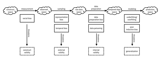
Figure 10.1. Bias in measurement and sampling are the most obvious sources of unfairness in machine learning, but not the only ones. Accessible caption. A sequence of five spaces, each represented as a cloud. The construct space leads to the observed space via the measurement process. The observed space leads to the raw data space via the sampling process. The raw data space leads to the prepared data space via the data preparation process. The prepared data space leads to the prediction space via the modeling process. The measurement process contains social bias, which threatens construct validity. The sampling process contains representation bias and temporal bias, which threatens external validity. The data preparation process contains data preparation bias and data poisoning, which threaten internal validity. The modeling process contains underfitting/overfitting and poor inductive bias, which threaten generalization.
Social bias enters claims data in a few ways. First, you might think that patients who visit doctors a lot and get many prescriptions filled, i.e. utilize the health care system a lot, are sicker and thus more appropriate candidates for care management. While it is directionally true that greater health care utilization implies a sicker patient, it is not true when comparing patients across populations such as whites and blacks. Blacks tend to be sicker for an equal level of utilization due to structural issues in the health care system.[3] The same is true when looking at health care cost instead of utilization. Another social bias can be in the codes. For example, black people are less-often treated for pain than white people in the United States due to false beliefs among clinicians that black people feel less pain.[4] Moreover, there can be social bias in the human-determined labels of selection for care management in the past due to implicit cognitive biases or prejudice on the part of the decision maker. Representation bias enters claims data because it is only from Sospital’s own members. This population may, for example, undersample blacks if Sospital offers its commercial plans primarily in counties with larger white populations.
Besides the social and representation biases given above that are already present in raw data, you need to be careful that you don’t introduce other forms of unfairness in the problem specification and data preparation phases. For example, suppose you don’t have the labels from human decision makers in the past. In that case, you might decide to use a threshold on utilization or cost as a proxy outcome variable, but that would make blacks less likely to be selected for care management at equal levels of infirmity for the reasons described above. Also, as part of feature engineering, you might think to combine individual cost or utilization events into more comprehensive categories, but if you aren’t careful you could make racial bias worse. It turns out that combining all kinds of health system utilization into a single feature yields unwanted racial bias, but keeping inpatient hospital nights and frequent emergency room utilization as separate kinds of utilization keeps the bias down in nationally-representative data.[5]
“As AI is embedded into our day to day lives it’s critical that we ensure our models don’t inadvertently incorporate latent stereotypes and prejudices.”
—Richard Zemel, computer scientist at University of Toronto
You might be thinking that you already know how to measure and mitigate biases in measurement, sampling, and data preparation from Chapter 9, distribution shift. What’s different about fairness? Although there is plenty to share between distribution shift and fairness,[6] there are two main technical differences between the two topics. First is access to the construct space. You can get data from the construct space in distribution shift scenarios. Maybe not immediately, but if you wait, collect, and label data from the deployment environment, you will have data reflecting the construct space. However, you never have access to the construct space in fairness settings. The construct space reflects a perfect egalitarian world that does not exist in real life, so you can’t get data from it. (Recall that in Chapter 4, we said that hakuna matata reigns in the construct space (it means no worries).) Second is the specification of what is sought. In distribution shift, there is no further specification beyond just trying to match the shifted distribution. In fairness, there are precise policy-driven notions and quantitative criteria that define the desired state of data and/or models that are not dependent on the data distribution you have. You’ll learn about these precise notions and how to choose among them in the next chapter.
Related to causal and anticausal learning covered in Chapter 9, the protected attribute is like the environment variable. Fairness and distributive justice are usually conceived in a causal (rather than anticausal) learning framework in which the outcome label is extrinsic: the protected attribute may cause the other features, which in turn cause the selection for care management. However, this setup is not always the case.
10.3 Defining Group Fairness
You’ve gone back to the problem specification phase after some amount of data understanding because you and the problem owner have realized that there is a strong possibility of unfairness if left unchecked. Given the Section 1557 regulations Sospital is working under as a health insurer, you start by looking deeper into group fairness. Group fairness is about comparing members of the privileged group and members of the unprivileged group on average.
10.3.1 Statistical Parity Difference and Disparate Impact Ratio
One
key concept in unwanted discrimination is disparate impact:
privileged and unprivileged groups receiving different outcomes irrespective of
the decision maker’s intent and irrespective of the decision-making procedure. Statistical
parity difference is a group fairness metric that you can consider in the care
management problem specification that quantifies disparate impact by computing the
difference in selection rates of the favorable label ![]() (rate of receiving
extra care) between the privileged (
(rate of receiving
extra care) between the privileged (![]() ; whites) and
unprivileged groups (
; whites) and
unprivileged groups (![]() ; blacks):
; blacks):
![]()
Equation 10.1
A
value of ![]() means that members
of the unprivileged group (blacks) and the privileged group (whites) are
getting selected for extra care management at equal rates, which is considered
a fair situation. A negative value of statistical parity difference indicates
that the unprivileged group is at a disadvantage and a positive value indicates
that the privileged group is at a disadvantage. A requirement in a problem
specification may be that the learned model must have a statistical parity
difference close to
means that members
of the unprivileged group (blacks) and the privileged group (whites) are
getting selected for extra care management at equal rates, which is considered
a fair situation. A negative value of statistical parity difference indicates
that the unprivileged group is at a disadvantage and a positive value indicates
that the privileged group is at a disadvantage. A requirement in a problem
specification may be that the learned model must have a statistical parity
difference close to ![]() . An example
calculation of statistical parity difference is shown in Figure 10.2.
. An example
calculation of statistical parity difference is shown in Figure 10.2.
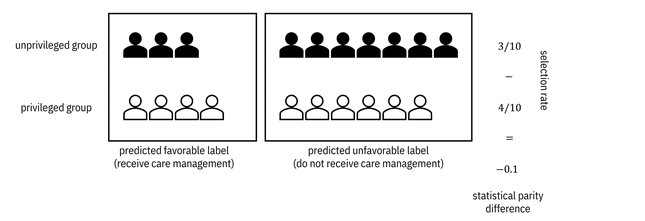
Figure 10.2. An example calculation of statistical parity
difference. Accessible caption. 3 members of the unprivileged group are
predicted with the favorable label (receive care management) and 7 are
predicted with the unfavorable label (don’t receive care management). 4 members
of the privileged group are predicted with the favorable label and 6 are
predicted with the unfavorable label. The selection rate for the unprivileged
group is ![]() and for the
privileged group is
and for the
privileged group is ![]() . The difference,
the statistical parity difference is
. The difference,
the statistical parity difference is ![]() .
.
Disparate impact can also be quantified as a ratio:
![]()
Equation 10.2
Here,
a value of ![]() indicates
fairness, values less than
indicates
fairness, values less than ![]() indicate
disadvantage faced by the unprivileged group, and values greater than
indicate
disadvantage faced by the unprivileged group, and values greater than ![]() indicate
disadvantage faced by the privileged group. The disparate
impact ratio is also sometimes known as the relative
risk ratio or the adverse impact ratio. In
some application domains such as employment, a value of the disparate impact
ratio less than
indicate
disadvantage faced by the privileged group. The disparate
impact ratio is also sometimes known as the relative
risk ratio or the adverse impact ratio. In
some application domains such as employment, a value of the disparate impact
ratio less than ![]() is considered
unfair and values greater than
is considered
unfair and values greater than ![]() are considered
fair. This so-called four-fifths rule problem
specification is asymmetric because it does not speak to disadvantage
experienced by the privileged group. It can be symmetrized by considering
disparate impact ratios between
are considered
fair. This so-called four-fifths rule problem
specification is asymmetric because it does not speak to disadvantage
experienced by the privileged group. It can be symmetrized by considering
disparate impact ratios between ![]() and
and ![]() to be fair. Statistical
parity difference and disparate impact ratio can be understood as measuring a
form of independence between the prediction
to be fair. Statistical
parity difference and disparate impact ratio can be understood as measuring a
form of independence between the prediction ![]() and the protected
attribute
and the protected
attribute ![]() .[7]
Besides statistical parity difference and disparate impact ratio, another way
to quantify the independence between
.[7]
Besides statistical parity difference and disparate impact ratio, another way
to quantify the independence between ![]() and
and ![]() is their mutual
information.
is their mutual
information.
Both
statistical parity difference and disparate impact ratio can also be defined on
the training data instead of the model predictions by replacing ![]() with
with ![]() . Thus, they can be
measured and tested (1) on the dataset before model training, as a dataset fairness metric, as well as (2) on the learned
classifier after model training as a classifier fairness
metric, shown in Figure 10.3.
. Thus, they can be
measured and tested (1) on the dataset before model training, as a dataset fairness metric, as well as (2) on the learned
classifier after model training as a classifier fairness
metric, shown in Figure 10.3.
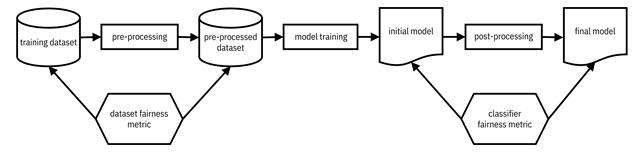
Figure 10.3. Two types of fairness metrics in different parts of the machine learning pipeline. Accessible caption. A block diagram with a training dataset as input to a pre-processing block with a pre-processed dataset as output. The pre-processed dataset is input to a model training block with an initial model as output. The initial model is input to a post-processing block with a final model as output. A dataset fairness metric block is applied to the training dataset and pre-processed dataset. A classifier fairness metric block is applied to the initial model and final model.
10.3.2 Average Odds Difference
You’ve examined disparate impact-based group fairness metrics so far, but want to learn another one before you start comparing and contrasting them as you figure out the problem specification for the care management model. A different group fairness metric is average odds difference, which is based on model performance metrics rather than simply the selection rate. (It can thus only be used as a classifier fairness metric, not a dataset fairness metric as shown in Figure 10.3.) The average odds difference involves the two metrics in the ROC: the true favorable label rate (true positive rate) and the false favorable label rate (false positive rate). You take the difference of true favorable rates between the unprivileged and privileged groups and the difference of the false favorable rates between the unprivileged and privileged groups, and average them:
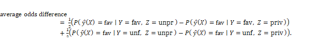
Equation 10.3
An example calculation of average odds difference is shown in Figure 10.4.
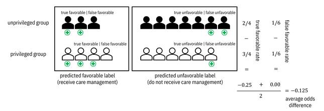
Figure 10.4. An example calculation of average odds
difference. The crosses below the members indicate a true need for care
management. Accessible caption. In the unprivileged group, 2 members
receive true favorable outcomes and 2 receive false unfavorable outcomes,
giving a ![]() true favorable
rate. In the privileged group, 3 members receive true favorable outcomes and 1
receives a false unfavorable outcome, giving a
true favorable
rate. In the privileged group, 3 members receive true favorable outcomes and 1
receives a false unfavorable outcome, giving a ![]() true favorable
rate. The true favorable rate difference is
true favorable
rate. The true favorable rate difference is ![]() . In the
unprivileged group, 1 member receives a false favorable outcome and 5 receive a
true unfavorable outcome, giving a
. In the
unprivileged group, 1 member receives a false favorable outcome and 5 receive a
true unfavorable outcome, giving a ![]() false favorable
rate. In the privileged group, 1 member receives a false favorable outcome and
5 receive a true unfavorable outcome, giving a
false favorable
rate. In the privileged group, 1 member receives a false favorable outcome and
5 receive a true unfavorable outcome, giving a ![]() false favorable
rate. The false favorable rate difference is
false favorable
rate. The false favorable rate difference is ![]() . Averaging the two
differences gives a
. Averaging the two
differences gives a ![]() average odds
difference.
average odds
difference.
In the average odds difference, the true favorable rate difference and the false favorable rate difference can cancel out and hide unfairness, so it is better to take the absolute value before averaging:
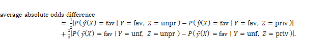
Equation 10.3
The
average odds difference is a way to measure the separation
of the prediction ![]() and the protected
attribute
and the protected
attribute ![]() by the true label
by the true label ![]() in any of the
three Bayesian networks shown in Figure 10.5. A value of
in any of the
three Bayesian networks shown in Figure 10.5. A value of ![]() average absolute odds
difference indicates independence of
average absolute odds
difference indicates independence of ![]() and
and ![]() conditioned on
conditioned on ![]() . This is deemed a
fair situation and termed equality of odds.
. This is deemed a
fair situation and termed equality of odds.

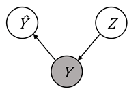

Figure 10.5. Illustration of the true label ![]() separating the
prediction and the protected attribute in various Bayesian networks. Accessible
caption. Three networks that show separation:
separating the
prediction and the protected attribute in various Bayesian networks. Accessible
caption. Three networks that show separation: ![]() à
à ![]() à
à ![]() ,
, ![]() ß
ß ![]() ß
ß ![]() , and
, and ![]() ß
ß ![]() à
à ![]() .
.
10.3.3 Choosing Between Statistical Parity and Average Odds Difference
What’s the point of these two different group fairness metrics? They don’t appear to be radically different. But they actually are radically different in an important conceptual way: either you believe there is social bias during measurement or not. These two worldviews have been named (1) “we’re all equal” (the privileged group and unprivileged group have the same inherent distribution of health in the construct space, but there is bias during measurement that makes it appear this is not the case) and (2) “what you see is what you get” (there are inherent differences between the two groups in the construct space and this shows up in the observed space without a need for any bias during measurement).[8] Since under the “we’re all equal” worldview, there is already structural bias in the observed space (blacks have lower health utilization and cost for the same level of health as whites), it does not really make sense to look at model accuracy rates computed in an already-biased space. Therefore, independence or disparate impact fairness definitions make sense and your problem specification should be based on them. However, if you believe that “what you see is what you get”—the observed space is a true representation of the inherent distributions of the groups and the only bias is sampling bias—then the accuracy-related equality of odds fairness metrics make sense. In this case, your problem specification should be based on equality of odds.
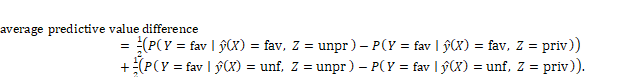
10.3.4 Average Predictive Value Difference
And
if it wasn’t complicated enough, let’s throw one more group fairness definition
into the mix: calibration by group or sufficiency. Recall from Chapter 6 that for continuous
score outputs, the predicted score corresponds to the proportion of positive true
labels in a calibrated classifier, or ![]() . For fairness,
you’d like the calibration to be true across the groups defined by protected
attributes, so
. For fairness,
you’d like the calibration to be true across the groups defined by protected
attributes, so ![]() for all groups
for all groups ![]() . If a classifier
is calibrated by group, it is also sufficient, which
means that
. If a classifier
is calibrated by group, it is also sufficient, which
means that ![]() and
and ![]() conditioned on
conditioned on ![]() (or
(or ![]() ) are independent.
The graphical models for sufficiency are shown in Figure 10.6. To allow for
better comparison to Figure 10.5 (the graphical models of separation), the
predicted score is indicated by
) are independent.
The graphical models for sufficiency are shown in Figure 10.6. To allow for
better comparison to Figure 10.5 (the graphical models of separation), the
predicted score is indicated by ![]() rather than
rather than ![]() .
.

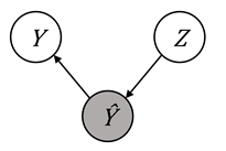
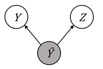
Figure 10.6. Illustration of the predicted label ![]() separating the
true label and the protected attribute in various Bayesian networks, which is
known as sufficiency. Accessible caption. Three networks that show sufficiency:
separating the
true label and the protected attribute in various Bayesian networks, which is
known as sufficiency. Accessible caption. Three networks that show sufficiency: ![]() à
à ![]() à
à ![]() ,
, ![]() ß
ß ![]() ß
ß ![]() , and
, and ![]() ß
ß ![]() à
à ![]() .
.
Since
sufficiency and separation are somewhat opposites of each other with ![]() and
and ![]() reversed, their
quantifications are also opposites with
reversed, their
quantifications are also opposites with ![]() and
and ![]() reversed. Recall from
Chapter 6 that the positive predictive value is the reverse of the true
positive rate:
reversed. Recall from
Chapter 6 that the positive predictive value is the reverse of the true
positive rate: ![]() and that the false
omission rate is the reverse of the false positive rate:
and that the false
omission rate is the reverse of the false positive rate: ![]() . To quantify
sufficiency unfairness, compute the average difference of the positive
predictive value and false omission rate across the unprivileged (black) and
privileged (white) groups:
. To quantify
sufficiency unfairness, compute the average difference of the positive
predictive value and false omission rate across the unprivileged (black) and
privileged (white) groups:
Equation 10.4
An example calculation for average predictive value difference is shown in Figure 10.7. The example illustrates a case in which the two halves of the metric cancel out because they have opposite sign, so a version with absolute values before averaging makes sense:
Equation 10.5
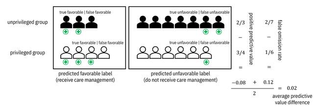
Figure 10.7. An example calculation of average predictive
value difference. The crosses below the members indicate a true need for care
management. Accessible caption. In the unprivileged group, 2 members
receive true favorable outcomes and 1 receives a false unfavorable outcome,
giving a ![]() positive
predictive value. In the privileged group, 3 members receive true favorable
outcomes and 1 receives a false unfavorable outcome, giving a
positive
predictive value. In the privileged group, 3 members receive true favorable
outcomes and 1 receives a false unfavorable outcome, giving a ![]() positive
predictive value. The positive predictive value difference is
positive
predictive value. The positive predictive value difference is ![]() . In the
unprivileged group, 2 members receive a false unfavorable outcome and 5 receive
a true unfavorable outcome, giving a
. In the
unprivileged group, 2 members receive a false unfavorable outcome and 5 receive
a true unfavorable outcome, giving a ![]() false omission
rate. In the privileged group, 1 member receives a false unfavorable outcome
and 5 receive a true unfavorable outcome, giving a
false omission
rate. In the privileged group, 1 member receives a false unfavorable outcome
and 5 receive a true unfavorable outcome, giving a ![]() false omission
rate. The false omission rate difference is
false omission
rate. The false omission rate difference is ![]() . Averaging the two
differences gives a
. Averaging the two
differences gives a ![]() average predictive
value difference.
average predictive
value difference.
10.3.5 Choosing Between Average Odds and Average Predictive Value Difference
What’s the difference between separation and sufficiency? Which one makes more sense for the Sospital care management model? This is not a decision based on politics and worldviews like the decision between independence and separation. It is a decision based on what the favorable label grants the affected user: is it assistive or simply non-punitive?[9] Getting a loan is assistive, but not getting arrested is non-punitive. Receiving care management is assistive. In assistive cases like receiving extra care, separation (equalized odds) is the preferred fairness metric because it relates to recall (true positive rate), which is of primary concern in these settings. If receiving care management had been a non-punitive act, then sufficiency (calibration) would have been the preferred fairness metric because precision is of primary concern in non-punitive settings. (Precision is equivalent to positive predictive value, which is one of the two components of the average predictive value difference.).
10.3.6 Conclusion
You can construct all sorts of different group fairness metrics by computing differences or ratios of the various confusion matrix entries and other classifier performance metrics detailed in Chapter 6, but independence, separation, and sufficiency are the three main ones. They are summarized in Table 10.1.
Table 10.1. The three main types of group fairness metrics.
|
Type |
Statistical Relationship |
Fairness Metric |
Can Be A Dataset Metric? |
Social Bias in Measurement |
Favorable Label |
|
independence |
|
statistical parity difference |
yes |
yes |
assistive or non-punitive |
|
separation |
|
average odds difference |
no |
no |
assistive |
|
sufficiency (calibration) |
|
average predictive value difference |
no |
no |
non-punitive |
Based on the different properties of the three group fairness metrics, and the likely social biases in the data you’re using to create the Sospital care management model, you should focus on independence and statistical parity difference.
10.4 Defining Individual and Counterfactual Fairness
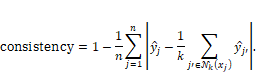
An important concept in fairness is intersectionality. Things might look fair when you look at different protected attributes separately, but when you define unprivileged groups as the intersection of multiple protected attributes, such as black women, group fairness metrics show unfairness. You can imagine making smaller and smaller groups by including more and more attributes, all the way to a logical end of groups that are just individuals that share all of their feature values. At this extreme, the group fairness metrics described in the previous section are no longer meaningful and a different notion of sameness is needed. That notion is individual fairness or consistency: that all individuals with the same feature values should receive the same predicted label and that individuals with similar features should receive similar predicted labels.
10.4.1 Consistency
The consistency metric is quantified as follows:
Equation 10.6
For
each of the ![]() Sospital members,
the prediction
Sospital members,
the prediction ![]() is compared to the
average prediction of the
is compared to the
average prediction of the ![]() nearest neighbors.
When the predicted labels of all of the
nearest neighbors.
When the predicted labels of all of the ![]() nearest neighbors
match the predicted label of the person themselves, you get . If all of the nearest neighbor
predicted labels are different from the predicted label of the person, the absolute value is
nearest neighbors
match the predicted label of the person themselves, you get . If all of the nearest neighbor
predicted labels are different from the predicted label of the person, the absolute value is ![]() . Overall, because
of the ‘one minus’ at the beginning of Equation 10.6, the consistency metric is
. Overall, because
of the ‘one minus’ at the beginning of Equation 10.6, the consistency metric is
![]() if all similar
points have similar labels and less than
if all similar
points have similar labels and less than ![]() if similar points
have different labels.
if similar points
have different labels.
The biggest question in individual fairness is deciding the distance metric by which the nearest neighbors are determined. Which kind of distance makes sense? Should all features be used in the distance computation? Should protected attributes be excluded? Should some feature dimensions be corrected for in the distance computation? These choices are where politics and worldviews come into play.[10] Typically, protected attributes are excluded, but they don’t have to be. If you believe there is no bias during measurement (the “what you see is what you get” worldview), then you should simply use the features as is. In contrast, suppose you believe that there are structural social biases in measurement (the “we’re all equal” worldview). In that case, you should attempt to undo those biases by correcting the features as they’re fed into a distance computation. For example, if you believe that blacks with three outpatient doctor visits are equal in health to whites with five outpatient doctor visits, then your distance metric can add two outpatient visits to the black members as a correction.
10.4.2 Counterfactual Fairness
One
special case of individual fairness is when two patients have exactly the same
feature values and only differ in one protected attribute. Think of two
patients, one black and one white who have an identical history of interaction
with the health care system. The situation is deemed fair if both receive the
same predicted label—either both are given extra care management or both are
not given extra care management—and unfair otherwise. Now take this special
case a step further. As a thought experiment, imagine an intervention ![]() that changes the
protected attribute of a Sospital member from black to white or vice versa. If
the predicted label remains the same for all members, the classifier is counterfactually fair.[11]
(Actually intervening to change a member’s protected attribute is usually not
possible immediately, but this is just a thought experiment.) Counterfactual
fairness can be tested using treatment effect estimation methods from Chapter 8.
that changes the
protected attribute of a Sospital member from black to white or vice versa. If
the predicted label remains the same for all members, the classifier is counterfactually fair.[11]
(Actually intervening to change a member’s protected attribute is usually not
possible immediately, but this is just a thought experiment.) Counterfactual
fairness can be tested using treatment effect estimation methods from Chapter 8.
Protected attributes causing different outcomes across groups is an important consideration in many laws and regulations.[12] Suppose you have a full-blown causal graph of all the variables given to you or you discover one from data using the methods of Chapter 8. In that case, you can see which variables have causal paths to the label nodes, either directly or passing through other variables. If any of the variables with causal paths to the label are considered protected attributes, you have a fairness problem to investigate and mitigate.
10.4.3 Theil Index
If
you don’t want to decide between group and individual fairness metrics as
you’re figuring out the Sospital care management problem specification, do you have
any other options? Yes you do. You can use the Theil index, which was first
introduced in Chapter 3 as a summary statistic for uncertainty. It naturally
combines both individual and group fairness considerations. Remember from that
chapter that the Theil index was originally developed to measure the
distribution of wealth in a society. A value of ![]() indicates a
totally unfair society where one person holds all the wealth and a value of
indicates a
totally unfair society where one person holds all the wealth and a value of ![]() indicates an
egalitarian society where all people have the same amount of wealth.
indicates an
egalitarian society where all people have the same amount of wealth.
What
is the equivalent of wealth in the context of machine learning and distributive
justice in health care management? It has to be some sort of non-negative
benefit value ![]() that you want to
be equal for different Sospital members. Once you’ve defined the benefit
that you want to
be equal for different Sospital members. Once you’ve defined the benefit ![]() , plug it into the
Theil index expression and use it as a combined group and individual fairness metric:
, plug it into the
Theil index expression and use it as a combined group and individual fairness metric:
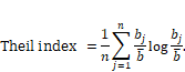
Equation 10.7
The
equation averages the benefit divided by the mean benefit ![]() , multiplied by its
natural log, across all people.
, multiplied by its
natural log, across all people.
That’s
all well and good, but benefit to who and under which worldview? The research group
that proposed using the Theil index in algorithmic fairness suggested that ![]() be
be ![]() for false
favorable labels (false positives),
for false
favorable labels (false positives), ![]() for true favorable
labels (true positives),
for true favorable
labels (true positives), ![]() for true
unfavorable labels (true negatives), and
for true
unfavorable labels (true negatives), and ![]() for false
unfavorable labels (false negatives).[13]
This recommendation is seemingly consistent with the “what you see is what you
get” worldview because it is examining model performance, assumes the costs of
false positives and false negatives are the same, and takes the perspective of
affected members who want to get care management even if they are not truly
suitable candidates. More appropriate benefit functions for the problem
specification of the Sospital model may be
for false
unfavorable labels (false negatives).[13]
This recommendation is seemingly consistent with the “what you see is what you
get” worldview because it is examining model performance, assumes the costs of
false positives and false negatives are the same, and takes the perspective of
affected members who want to get care management even if they are not truly
suitable candidates. More appropriate benefit functions for the problem
specification of the Sospital model may be ![]() that are (1)
that are (1) ![]() for true favorable
and true unfavorable labels and
for true favorable
and true unfavorable labels and ![]() for false favorable
and false unfavorable labels (“what you see is what you get” while balancing
societal needs), or (2)
for false favorable
and false unfavorable labels (“what you see is what you get” while balancing
societal needs), or (2) ![]() for true favorable
and false favorable labels and
for true favorable
and false favorable labels and ![]() for true
unfavorable and false unfavorable labels (“we’re all equal”).
for true
unfavorable and false unfavorable labels (“we’re all equal”).
10.4.4 Conclusion
Individual fairness consistency and Theil index are both excellent ways to capture various nuances of fairness in different contexts. Just like group fairness metrics, they require you to clarify your worldview and aim for the same goals in a bottom-up way. Since the Sospital care management setting is regulated using group fairness language, it behooves you to use group fairness metrics in your problem specification and modeling. Counterfactual or causal fairness is a strong requirement from the perspective of the philosophy and science of law, but the regulations are only just catching up. So you might need to utilize causal fairness in problem specifications in the future, but not just yet. As you’ve learned so far, the problem specification and data phases are critical for fairness. But that makes the modeling phase no less important. The next section focuses on bias mitigation to improve fairness as part of the modeling pipeline.
10.5 Mitigating Unwanted Bias
From
the earlier phases of the lifecycle of the Sospital care management model, you
know that you must address unwanted biases during the modeling phase. Given the
quantitative definitions of fairness and unfairness you’ve worked through, you
know that mitigating bias entails introducing some sort of statistical
independence between protected attributes like race and true or predicted
labels of needing care management. That sounds easy enough, so what’s the
challenge? What makes bias mitigation difficult is that other regular
predictive features ![]() have statistical
dependencies with the protected attributes and the labels (a node for
have statistical
dependencies with the protected attributes and the labels (a node for ![]() was omitted from Figure
10.5 and Figure 10.6, but out-of-sight does not mean out-of-mind). The regular
features can reconstruct the information contained in the protected attributes
and introduce dependencies, even if you do the most obvious thing of dropping
the protected attributes from the data. For example, race can be strongly
associated both with certain health care providers (some doctors have
predominantly black patients and other doctors have predominantly white
patients) and with historical selection for extra care management.
was omitted from Figure
10.5 and Figure 10.6, but out-of-sight does not mean out-of-mind). The regular
features can reconstruct the information contained in the protected attributes
and introduce dependencies, even if you do the most obvious thing of dropping
the protected attributes from the data. For example, race can be strongly
associated both with certain health care providers (some doctors have
predominantly black patients and other doctors have predominantly white
patients) and with historical selection for extra care management.
Bias mitigation methods must be more clever than simply dropping protected attributes. Don’t take a shortcut: dropping protected attributes is never the right answer. Remember the two main ways of mitigating the ills of distribution shift in Chapter 9: adaptation and min-max robustness. When applied to bias mitigation, adaptation-based techniques are much more common than robustness-based ones, but rely on having protected attributes in the training dataset.[14] They are the subject of the remainder of this section. If the protected attributes are not available in the training data, min-max robustness techniques for fairness that mirror those for distribution shift can be used.[15]
Figure 10.8 (a subset of Figure 10.3) shows three different points of intervention for bias mitigation: (1) pre-processing which alters the statistics of the training data, (2) in-processing which adds extra constraints or regularization terms to the learning process, and (3) post-processing which alters the output predictions to make them more fair. Pre-processing can only be done when you have the ability to touch and modify the training data. Since in-processing requires you to mess with the learning algorithm, it is the most involved and least flexible. Post-processing is almost always possible and the easiest to pull off. However, the earlier in the pipeline you are, the more effective you can be.
There are several specific methods within each of the three categories of bias mitigation techniques (pre-processing, in-processing, post-processing). Just like for accuracy, no one best algorithm outperforms all other algorithms on all datasets and fairness metrics (remember the no free lunch theorem). Just like there are differing domains of competence for classifiers covered in Chapter 7, there are differing domains of competence for bias mitigation algorithms. However, fairness is a new field that has not yet been studied extensively enough to have good characterizations of those domains of competence yet. In Chapter 7, it was important to go down into the details of machine learning methods because that understanding is used in this and other later chapters. The reason to dive into the details of bias mitigation algorithms is different. In choosing a bias mitigation algorithm, you have to (1) know where in the pipeline you can intervene, (2) consider your worldview, and (3) understand whether protected attributes are allowed as features and will be available in the deployment data when you are scoring new Sospital members.
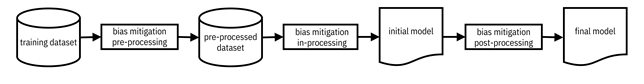
Figure 10.8. Three types of bias mitigation algorithms in different parts of the machine learning pipeline. Accessible caption. A block diagram with a training dataset as input to a bias mitigation pre-processing block with a pre-processed dataset as output. The pre-processed dataset is input to a bias mitigation in-processing block with an initial model as output. The initial model is input to a bias mitigation post-processing block with a final model as output.
10.5.1 Pre-Processing
At the pre-processing stage of the modeling pipeline, you don’t have the trained model yet. So pre-processing methods cannot explicitly include fairness metrics that involve model predictions. Therefore, most pre-processing methods are focused on the “we’re all equal” worldview, but not exclusively so. There are several ways for pre-processing a training data set: (1) augmenting the dataset with additional data points, (2) applying instance weights to the data points, and (3) altering the labels.
One of the simplest algorithms for pre-processing the training dataset is to append additional rows of made-up members that do not really exist. These imaginary members are constructed by taking existing member rows and flipping their protected attribute values (like counterfactual fairness).[16] The augmented rows are added sequentially based on a distance metric so that ‘realistic’ data points close to modes of the underlying dataset are added first. This ordering maintains the fidelity of the data distribution for the learning task. A plain uncorrected distance metric takes the “what you see is what you get” worldview and only overcomes sampling bias, not measurement bias. A corrected distance metric like the example described in the previous section (adding two outpatient visits to the black members) takes the “we’re all equal” worldview and can overcome both measurement and sampling bias (threats to both construct and external validity). This data augmentation approach needs to have protected attributes as features of the model and they must be available in deployment data.
Another way to pre-process the training data set is through sample weights, similar to inverse probability weighting and importance weighting seen in Chapter 8 and Chapter 9, respectively. The reweighing method is geared toward improving statistical parity (“we’re all equal” worldview), which can be assessed before the care management model is trained and is a dataset fairness metric.[17] The goal of independence between the label and protected attribute corresponds to their joint probability being the product of their marginal probabilities. This product probability appears in the numerator and the actual observed joint probability appears in the denominator of the weight:
![]()
Equation 10.8
Protected attributes are required in the training data to learn the model, but they don’t have to be part of the model or the deployment data.
Whereas data augmentation and reweighing do not change the training data you have from historical care management decisions, other methods do. One simple method, only for statistical parity and the “we’re all equal” worldview, known as massaging flips unfavorable labels of unprivileged group members to favorable labels and favorable labels of privileged group members to unfavorable labels.[18] The chosen data points are those closest to the decision boundary that have low confidence. Massaging does not need to have protected attributes in the deployment data.
A
different approach, the fair score transformer, works
on (calibrated) continuous score labels ![]() rather than binary
labels.[19]
It is posed as an optimization in which you find transformed scores
rather than binary
labels.[19]
It is posed as an optimization in which you find transformed scores ![]() that have small
cross-entropy with the original scores
that have small
cross-entropy with the original scores ![]() , i.e.
, i.e. ![]() , while
constraining the statistical parity difference, average odds difference, or
other group fairness metrics of your choice to be of small absolute value. You
convert the pre-processed scores back into binary labels with weights to feed
into a standard training algorithm. You can take the “what you see is what you
get” worldview with the fair score transformer because it assumes that the
classifier later trained on the pre-processed dataset is competent, so that the
pre-processed score it produces is a good approximation to the score predicted
by the trained model. Although there are pre-processing methods that alter both
the labels and (structured or semi-structured) features,[20]
the fair score transformer proves that you only need to alter the labels. It
can deal with deployment data that does not come with protected attributes.
, while
constraining the statistical parity difference, average odds difference, or
other group fairness metrics of your choice to be of small absolute value. You
convert the pre-processed scores back into binary labels with weights to feed
into a standard training algorithm. You can take the “what you see is what you
get” worldview with the fair score transformer because it assumes that the
classifier later trained on the pre-processed dataset is competent, so that the
pre-processed score it produces is a good approximation to the score predicted
by the trained model. Although there are pre-processing methods that alter both
the labels and (structured or semi-structured) features,[20]
the fair score transformer proves that you only need to alter the labels. It
can deal with deployment data that does not come with protected attributes.
Data augmentation, reweighing, massaging, and fair score transformer all have their own domains of competence. Some perform better than others on different fairness metrics and dataset characteristics. You’ll have to try different ones to see what happens on the Sospital data.
10.5.2 In-Processing
In-processing bias mitigation algorithms are straightforward to state, but often more difficult to actually optimize. The statement is as follows: take an existing risk minimization supervised learning algorithm, such as (a repetition of Equation 7.4):
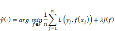
Equation 10.9
and
regularize or constrain it using a fairness metric. The algorithm can be
logistic regression and the regularizer can be statistical parity difference,
in which case you have the prejudice remover.[21]
More recent fair learning algorithms are broader and allow for any standard
risk minimization algorithm along with a broad set of group fairness metrics as
constraints that cover the different types of fairness.[22]
A recent in-processing algorithm regularizes the objective function using a
causal fairness term. Under strong ignorability assumptions (remember from Chapter
8 that these are no unmeasured confounders and overlap), the regularizer is an
average treatment effect-like term ![]() .[23]
.[23]
Once trained, the resulting models can be used on new unseen Sospital members. These in-processing algorithms do not require the deployment data to contain the protected attribute. The trick with all of them is structuring the bias mitigating regularization term or constraint so that the objective function can tractably be minimized through an optimization algorithm.
10.5.3 Post-Processing
If
you’re in the situation that the Sospital care management model has already
been trained and you cannot change it or touch the training data (for example
if you are purchasing a pre-trained model from a vendor to include in your
pipeline), then the only option you have is to mitigate unwanted biases using
post-processing. You can only alter the output predictions ![]() to meet the group
fairness metrics you desire based on your worldview (i.e. flipping the
predicted labels from receiving care management to not receiving care
management and vice versa). If you have some validation data with labels, you
can post-process with the “what you see is what you get” worldview. You can
always post-process with the “we’re all equal” worldview, with or without
validation data.
to meet the group
fairness metrics you desire based on your worldview (i.e. flipping the
predicted labels from receiving care management to not receiving care
management and vice versa). If you have some validation data with labels, you
can post-process with the “what you see is what you get” worldview. You can
always post-process with the “we’re all equal” worldview, with or without
validation data.
Since group fairness metrics are computed on average, flipping any random member’s label within a group is the same as flipping any other random member’s.[24] A random selection of people, however, seems to be procedurally unfair. To overcome this issue, similar to massaging, you can prioritize flipping the labels of members whose data points are near the decision boundary and are thus low confidence samples.[25] You can also choose people within a group so that you reduce individual counterfactual unfairness.[26] All of these approaches require the protected attribute in the deployment data.
The fair score transformer described in the pre-processing section also has a post-processing version, which does not require the protected attribute and should be considered the first choice algorithm in the category of post-processing bias mitigation if the base classifier outputs continuous scores. It performs well empirically and is not computationally-intensive. Just like the pre-processing version, the idea is to find an optimal transformation of the predicted score output into a new score, which can then be thresholded to a binary prediction for the final care management decision that Sospital makes.
10.5.4 Conclusion
All of the different bias mitigation algorithms are options as you’re deciding what to finally do in the care management modeling pipeline. The things you have to think about are:
1. where in the pipeline can you make alterations (this will determine the category pre-, in-, or post-processing)
2. which worldview you’ve decided with the problem owner (this will disallow some algorithms that don’t work for the worldview you’ve decided)
3. whether the deployment data contains the protected attributes (if not, this will disallow some algorithms that require them).
These different decision points are summarized in Table 10.2. After that, you can just go with the algorithm that gives you the best quantitative results. But what is best? It is simply the pipeline with the best value for the fairness metric you’ve chosen in your problem specification.
But you might ask, shouldn’t I consider a tradeoff of fairness and accuracy when I choose the pipeline? Balancing tradeoffs and relationships among different elements of trustworthy machine learning is more fully covered in Chapter 14, but before getting there, it is important to note one important point. Even though it is a convenient shortcut, measuring classification accuracy on data from the prepared data space, which already contains social bias, representation bias, and data preparation bias is not the right thing to do. Just like you should measure performance of distribution shift adaptation on data from the new environment—its construct space, you should measure accuracy after bias mitigation in its construct space where there is no unfairness. There is a tradeoff between fairness and accuracy measured in the prepared data space, but importantly there is no tradeoff between accuracy and fairness in the construct space.[27] You can approximate a construct space test set by using the data augmentation pre-processing method.
Table 10.2. Characteristics of the main bias mitigation algorithms.
|
Algorithm |
Category |
Fairness |
Protected Attributes in Deployment Data |
|
data augmentation |
pre |
counterfactual |
yes |
|
reweighing |
pre |
independence |
no |
|
massaging |
pre |
independence |
no |
|
fair score transformer |
pre, post |
independence, separation |
no |
|
prejudice remover |
in |
independence |
no |
|
recent in-processing algorithms |
in |
independence, separation, sufficiency |
no |
|
causal regularizer |
in |
counterfactual |
no |
|
group fairness post-processing |
post |
independence, separation |
yes |
|
individual and group fairness post-processing |
post |
counterfactual, independence, separation |
yes |
In your Sospital problem, you have almost complete flexibility because you do control the training data and model training, are focused on independence and the “we’re all equal” worldview, and are able to include protected attributes for Sospital’s members in the deployment data. Try everything, but start with the fair score transformer pre-processing.
10.6 Other Considerations
Before concluding the chapter, let’s consider a couple other issues. The first did not come up in the Sospital care management use case, but can come up in other use cases. The Sospital problem lent itself to fairness in the context of direct allocation decisions, but that is not the only possibility. There are also harms in representation or quality-of-service, such as bias in search results. For example, image searches for professions might yield only white people, web search results for personal names overrepresented in the black community might be accompanied by advertisements for criminal defense attorneys, and natural language processing algorithms for language translation or query understanding might associate doctors with men and nurses with women automatically. Some of the bias mitigation algorithms for allocative fairness can be used in representational fairness, but different techniques may be more appropriate.
“Most of this work is narrow in scope, focusing on fine-tuning specific models, making datasets more inclusive/representative, and ‘debiasing’ datasets. Although such work can constitute part of the remedy, a fundamentally equitable path must examine the wider picture, such as unquestioned or intuitive assumptions in datasets, current and historical injustices, and power asymmetries.”
—Abeba Birhane, cognitive scientist at University College Dublin
“I continue to worry that in CS (as in psychology), debates about bias have become a powerful distraction—drawing attention away from what's most important toward what's more easily measurable.”
—J. Nathan Matias, behavioral scientist at Cornell University
The second issue is as follows. Have we too easily swept the important considerations of algorithmic fairness under the rug of mathematics? Yes and no. If you have truly thought through the different sources of inequity arising throughout the machine learning lifecycle utilizing a panel of diverse voices, then applying the quantitative metrics and mitigation algorithms is actually pretty straightforward. It is straightforward because of the hard work you’ve done before getting to the modeling phase of the lifecycle and you should feel confident in going forward. If you have not done the hard work earlier in the lifecycle (including problem specification), blindly applying bias mitigation algorithms might not reduce harms and can even exacerbate them. So don’t take shortcuts.
10.7 Summary
§ Fairness has many forms, arising from different kinds of justice. Distributive justice is the most appropriate for allocation decisions made or supported by machine learning systems. It asks for some kind of sameness in the outcomes across individuals and groups.
§ Unfairness can arise from problem misspecification (including inappropriate proxy labels), feature engineering, measurement of features from the construct space to the observed space, and sampling of data points from the observed space to the raw data space.
§ There are two important worldviews in determining which kind of sameness is most appropriate for your problem.
§ If you believe there are social biases in measurement (not only representation biases in sampling), then you have the “we’re all equal” worldview; independence and statistical parity difference are appropriate notions of group fairness.
§ If you believe there are no social biases in measurement, only representation biases in sampling, then you have the “what you see is what you get” worldview; separation, sufficiency, average odds difference, and average predictive value difference are appropriate notions of group fairness.
§ If the favorable label is assistive, separation and average odds difference are appropriate notions of group fairness. If the favorable label is non-punitive, sufficiency and average predictive value difference are appropriate notions of group fairness.
§ Individual fairness is a limiting version of group fairness with finer and finer groups. Worldviews play a role in determining distance metrics between individuals.
§ Bias mitigation algorithms can be applied as pre-processing, in-processing, or post-processing within the machine learning pipeline. Different algorithms apply to different worldviews. The choice of algorithm should consider the worldview in addition to empirical performance.