1    

2    

3    

4    

5    

6    

7    

8    

9    

Distribution Shift

Wavetel is a leading (fictional) mobile telephony provider in India that expanded its operations to several East and Central African countries in recent years. One of its profit centers in the African markets is credit enabled by mobile money that it runs through partnerships with banks in each of the nations. The most straightforward application of mobile money is savings, first started in Kenya in 2007 under the name M-Pesa. With mobile money savings, customers can deposit, withdraw, and transfer funds electronically without a formal bank account, all through their mobile phones. (Remember that these transactions are one of the data sources that Unconditionally evaluated in Chapter 4.) More advanced financial services such as credit and insurance later emerged. In these advanced services, the bank takes on financial risk and can’t just hand out accounts without an application process and some amount of due diligence.

Having seen how profitable mobile money-enabled credit can be, Wavetel strongly lobbied for it to be allowed in its home country of India and has just seen the regulations signed into law. Partnering with the (fictional) Bank of Bulandshahr, Wavetel is ready to deploy this new service under the name Phulo. Based on market research, Wavetel and the Bank of Bulandshahr expect Phulo to receive tens of thousands of applications per day when first launched. They have to be ready to approve or deny those applications in near real-time. To deal with this load, imagine that they have hired your data science team as consultants to create a machine learning model that makes the decisions.

The task you face, approving and denying mobile phone-enabled loans for unbanked customers in India has never been done before. The Bank of Bulandshahr’s historical loan approval data will not be useful for making decisions on Phulo applicants. However, Wavetel has privacy-preserved data from mobile money-enabled credit systems in several East and Central African countries that it has the rights and consent to use in its India operations. Can you train the Phulo machine learning model using the African datasets? What could go wrong?

If you’re not careful, there’s a lot that could go wrong. You could end up creating a really harmful and unreliable system, because of the big lie of machine learning: the core assumption that training data and testing data is independent and identically distributed (i.i.d.). This is almost never true in the real world, where there tends to be some sort of difference in the probability distributions of the training data and the data encountered during the model’s deployment. This difference in distributions is known as distribution shift. A competent model that achieves high accuracy when tested through cross-validation might not maintain that competence in the real world. Too much epistemic uncertainty sinks the ship of even a highly risk-minimizing model.

“All bets are off if there is a distribution shift when the model is deployed. (There's always a distribution shift.)”

—Arvind Narayanan, computer scientist at Princeton University

This chapter begins Part 4 of the book on reliability and dealing with epistemic uncertainty, which constitutes the second of four attributes of trustworthiness (the others are basic performance, human interaction, and aligned purpose) as well as the second of two attributes of safety (the first is minimizing risk and aleatoric uncertainty). As shown in Figure 9.1, you’re halfway home to creating trustworthy machine learning systems!

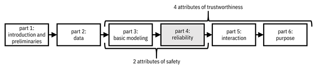
Figure 9.1. Organization of the book. This fourth part focuses on the second attribute of trustworthiness, reliability, which maps to machine learning models that are robust to epistemic uncertainty. Accessible caption. A flow diagram from left to right with six boxes: part 1: introduction and preliminaries; part 2: data; part 3: basic modeling; part 4: reliability; part 5: interaction; part 6: purpose. Part 4 is highlighted. Parts 3–4 are labeled as attributes of safety. Parts 3–6 are labeled as attributes of trustworthiness.

In this chapter, while working through the modeling phase of the machine learning lifecycle to create a safe and reliable Phulo model, you will:

§  examine how epistemic uncertainty leads to poor machine learning models, both with and without distribution shift,

§  judge which kind of distribution shift you have, and

§  mitigate the effects of distribution shift in your model.

 

9.1           Epistemic Uncertainty in Machine Learning

You have the mobile money-enabled credit approval/denial datasets from East and Central African countries and want to train a reliable Phulo model for India. You know that for safety, you must worry about minimizing epistemic uncertainty: the possibility of unexpected harms. Chapter 3 taught you how to differentiate aleatoric uncertainty from epistemic uncertainty. Now’s the time to apply what you learned and figure out where epistemic uncertainty is rearing its head!

First, in Figure 9.2, let’s expand on the picture of the different biases and validities from Figure 4.3 to add a modeling step that takes you from the prepared data space to a prediction space where the output predictions of the model live. As you learned in Chapter 7, in modeling, you’re trying to get the classifier to generalize from the training data to the entire set of features by using an inductive bias, without overfitting or underfitting. Working backwards from the prediction space, the modeling process is the first place where epistemic uncertainty creeps in. Specifically, if you don’t have the information to select a good inductive bias and hypothesis space, but you could obtain it in principle, then you have epistemic uncertainty.[1] Moreover, if you don’t have enough high-quality data to train the classifier even if you have the perfect hypothesis space, you have epistemic uncertainty.

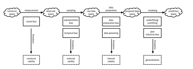
Figure 9.2. Different spaces and what can go wrong due to epistemic uncertainty throughout the machine learning pipeline. Accessible caption. A sequence of five spaces, each represented as a cloud. The construct space leads to the observed space via the measurement process. The observed space leads to the raw data space via the sampling process. The raw data space leads to the prepared data space via the data preparation process. The prepared data space leads to the prediction space via the modeling process. The measurement process contains social bias, which threatens construct validity. The sampling process contains representation bias and temporal bias, which threatens external validity. The data preparation process contains data preparation bias and data poisoning, which threaten internal validity. The modeling process contains underfitting/overfitting and poor inductive bias, which threaten generalization.

The epistemic uncertainty in the model has a few different names, including the Rashomon effect[2] and underspecification.[3] The main idea, illustrated in Figure 9.3, is that a lot of models perform similarly well in terms of aleatoric uncertainty and risk, but have different ways of generalizing because you have not minimized epistemic uncertainty. They all have the possibility of being competent and reliable models. They have a possibility value of . (Other models that do not perform well have a possibility value of  of being competent and reliable models.) However, many of these possible models are unreliable and they take shortcuts by generalizing from spurious characteristics in the data that people would not naturally think are relevant features to generalize from.[4] They are not causal. Suppose one of the African mobile money-enabled credit datasets just happens to have a spurious feature like the application being submitted on a Tuesday that predicts the credit approval label very well. In that case, a machine learning training algorithm will not know any better and will use it as a shortcut to fit the model. And you know that taking shortcuts is no-no for you when building trustworthy machine learning systems, so you don’t want to let your models take shortcuts either.

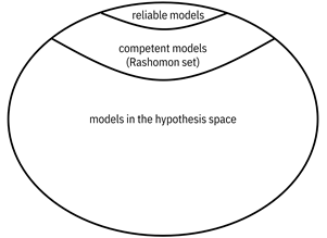
Figure 9.3. Among all the models you are considering, many of them can perform well in terms of accuracy and related measures; they are competent and constitute the Rashomon set. However, due to underspecification and the epistemic uncertainty that is present, many of the competent models are not safe and reliable. Accessible caption. A nested set diagram with reliable models being a small subset of competent models (Rashomon set), which are in turn a small subset of models in the hypothesis space.

How can you know that a competent high-accuracy model is one of the reliable, safe ones and not one of the unreliable, unsafe ones? The main way is to stress test it by feeding in data points that are edge cases beyond the support of the training data distribution. More detail about how to test machine learning systems in this way is covered in Chapter 13.

The main way to reduce epistemic uncertainty in the modeling step that goes from the prepared data space to the prediction space is data augmentation. If you can, you should collect more data from more environments and conditions, but that is probably not possible in your Phulo prediction task. Alternatively, you can augment your training dataset by synthetically generating training data points, especially those that push beyond the margins of the data distribution you have. Data augmentation can be done for semi-structured data modalities by flipping, rotating, and otherwise transforming the data points you have. In structured data modalities, like have with Phulo, you can create new data points by changing categorical values and adding noise to continuous values. However, be careful that you do not introduce any new biases in the data augmentation process.

 

9.2           Distribution Shift is a Form of Epistemic Uncertainty

So far, you’ve considered the epistemic uncertainty in going from the prepared data space to the prediction space by modeling, but there’s epistemic uncertainty earlier in the pipeline too. This epistemic uncertainty comes from all of the biases you don’t know about or don’t understand very well when going from the construct space to the prepared data space. We’ll come back to some of them in Chapter 10 and Chapter 11 when you learn how to make machine learning systems fair and adversarially robust. But for now, when building the Phulo model in India using data from several East and Central African countries, your most obvious source of epistemic uncertainty is sampling. You have sampled your data from a different time (temporal bias) and population (representation bias) than what Phulo is going to be deployed on. You might also have epistemic uncertainty in measurement: it is possible that the way creditworthiness shows up in India is different than in East and Central African countries because of cultural differences (social bias). Putting everything together, the distributions of the training data and the deployed data are not identical: . (Remember that  is features and  is labels.) You have distribution shift.

9.2.1        The Different Types of Distribution Shift

In building out the Phulo model, you know that the way you’ve measured and sampled the data in historical African contexts is mismatched with the situation in which Phulo will be deployed: present-day India. What are the different ways in which the training data distribution  can be different from the deployment data distribution ? There are three main ways.

1.    Prior probability shift, also known as label shift, is when the label distributions are different but the features given the labels are the same: [5] and .

2.    Covariate shift is the opposite, when the feature distributions are different but the labels given the features are the same:  and .

3.    Concept drift is when the labels given the features are different but the features are the same:  and , or when the features given the labels are different but the labels are the same:  and .

All other distribution shifts do not have special names like these three types. The first two types of distribution shift come from sampling differences whereas the third type of distribution shift comes from measurement differences. The three different types of distribution shift are summarized in Table 9.1.

Table 9.1. The three types of distribution shift.

Type	What Changes	What is the Same	Source	Threatens	Learning Problem
prior probability shift			sampling	external validity	anticausal learning
covariate shift			sampling	external validity	causal learning
concept drift			measurement	construct validity	causal learning
					anticausal learning

 

Let’s go through an example of each type to see which one (or more than one) affects the Phulo situation. There will be prior probability shift if there are different proportions of creditworthy people in present-day India and historical African countries, maybe because of differences in the overall economy. There will be covariate shift if the distribution of features is different. For example, maybe people in India have more assets in gold than in East and Central African countries. There will be concept drift if the actual mechanism connecting the features and creditworthiness is different. For example, people in India who talk or SMS with many people may be more creditworthy while in East and Central Africa, people who talk or SMS with few people may be more creditworthy.

One way to describe the different types of distribution shifts is through the context or environment. What does changing the environment in which the data was measured and sampled do to the features and label? And if you’re talking about doing, you’re talking about causality. If you treat the environment as a random variable , then the different types of distribution shifts have the causal graphs shown in Figure 9.4.[6]

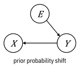
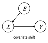
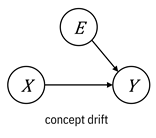
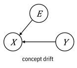
Figure 9.4. Causal graph representations of the different types of distribution shift. Accessible caption. Graphs of prior probability shift ( à  à ), covariate shift ( à  à ), concept drift ( à  ß ), and concept drift ( à  ß ).

These graphs illustrate a nuanced point. When you have prior probability shift, the label causes the feature and when you have covariate shift, the features cause the label. This is weird to think about, so let’s slow down and work through this concept. In the first case,  à , the label is known as an intrinsic label and the machine learning problem is known as anticausal learning. A prototypical example is a disease with a known pathogen like malaria that causes specific symptoms like chills, fatigue, and fever. The label of a patient having a disease is intrinsic because it is a basic property of the infected patient, which then causes the observed features. In the second case,  à , the label is known as an extrinsic label and the machine learning problem is known as causal learning. A prototypical example of this case is a syndrome, a collection of symptoms such as Asperger’s that isn’t tied to a pathogen. The label is just a label to describe the symptoms like compulsive behavior and poor coordination; it doesn’t cause the symptoms. The two different versions of concept drift correspond to anticausal and causal learning, respectively. Normally, in the practice of doing supervised machine learning, the distinction between anticausal and causal learning is just a curiosity, but it becomes important when figuring out what to do to mitigate the effect of distribution shift. It is not obvious which situation you’re in with the Phulo model, and you’ll have to really think about it.

9.2.2        Detecting Distribution Shift

Given that your training data is from East and Central African countries and your deployment data will come from India, you are aware that distribution shift probably exists in your modeling task. But how do you definitively detect it? There are two main ways:

1.    data distribution-based shift detection, and

2.    classifier performance-based shift detection,

that are applicable at two different points of the machine learning modeling pipeline, show in Figure 9.5.[7] Data distribution-based shift detection is done on the training data before the model training. Classifier performance-based shift detection is done afterwards on the model. Data distribution-based shift detection, as its name implies, directly compares  and  to see if they are similar or different. A common way is to compute their K-L divergence, which was introduced in Chapter 3. If it is too high, then there is distribution shift. Classifier performance-based shift detection examines the Bayes risk, accuracy, -score, or other model performance measure. If it is much poorer than the performance during cross-validation, there is distribution shift.

That is all well and good, but did you notice something about the two methods of distribution shift detection that make them unusable for your Phulo development task? They require the deployed distribution: both its features and labels. But you don’t have it! If you did, you would have used it to train the Phulo model. Shift detection methods are really meant for monitoring scenarios in which you keep getting data points to classify over time and you keep getting ground truth labels soon thereafter.

 

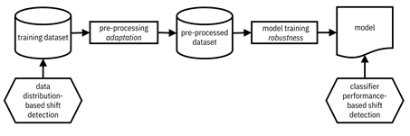
Figure 9.5. Modeling pipeline for detecting and mitigating distribution shift. Accessible caption. A block diagram with a training dataset as input to a pre-processing block labeled adaptation with a pre-processed dataset as output. The pre-processed dataset is input to a model training block labeled robustness with a model as output. A data distribution-based shift detection block is applied to the training dataset. A classifier performance-based shift detection block is applied to the model.

If you’ve started to collect unlabeled feature data from India, you can do unsupervised data distribution-based shift detection by comparing the India feature distribution to the Africa feature distributions. But you kind of already know that they’ll be different, and this unsupervised approach will not permit you to determine which type of distribution shift you have. Thus, in a Phulo-like scenario, you just have to assume the existence and type of distribution shift based on your knowledge of the problem. (Remember our phrase from Chapter 8: “those who can’t do, assume.”)

9.2.3        Mitigating Distribution Shift

There are two different scenarios when trying to overcome distribution shift to create a safe and trustworthy machine learning model: (1) you have unlabeled feature data  from the deployment distribution, which will let you adapt your model to the deployment environment, and (2) you have absolutely no data from the deployment distribution, so you must make the model robust to any deployment distribution you might end up encountering.

“Machine learning systems need to robustly model the range of situations that occur in the real-world.”

—Drago Anguelov, computer scientist at Waymo

The two approaches take place in different parts of the modeling pipeline shown in Figure 9.5. Adaptation is done on the training data as a pre-processing step, whereas robustness is introduced as part of the model training process. The two kinds of mitigation are summarized in Table 9.2.

Table 9.2. The two types of distribution shift mitigation.

Type	Where in the Pipeline	Known Deployment Environment	Approach for Prior Probability and Covariate Shifts	Approach for Concept Drift
adaptation	pre- processing	yes	sample weights	obtain labels
robustness	model training	no	min-max formulation	invariant risk minimization

 

The next sections work through adaptation and robustness for the different types of distribution shift. Mitigating prior probability shift and covariate shift is easier than mitigating concept drift because the relationship between the features and labels does not change in the first two types. Thus, the classifier you learned on the historical African training data continues to capture that relationship even on India deployment data; it just needs a little bit of tuning.

 

9.3           Adaptation

The first mitigation approach, adaptation, is done as a pre-processing of the training data from East and Central African countries using information available in unlabeled feature data  from India. To perform adaptation, you must know that India is where you’ll be deploying the model and you must be able to gather some features.

9.3.1        Prior Probability Shift

Since prior probability shift arises from sampling bias, the relationship between features and labels, and thus the ROC, does not change. Adapting is simply a matter of adjusting the classifier threshold or operating point based on the confusion matrix, which are all concepts you learned in Chapter 6. A straightforward and effective way to adapt to prior probability shift is a weighting scheme. The algorithm is as follows.[8]

1.    Train a classifier on one random split of the training data to get  and compute the classifier’s confusion matrix on another random split of the training data:
 .

2.     Run the unlabeled features of the deployment data through the classifier:  and compute the probabilities of positives and negatives in the deployment data as a vector:

.

3.    Compute weights . This is a vector of length two.

4.    Apply the weights to the training data points in the first random split and retrain the classifier. The first of the two weights multiplies the loss function of the training data points with label . The second of the two weights multiplies the loss function of the training data points with label .

The retrained classifier is what you want to use when you deploy Phulo in India under the assumption of prior probability shift.

9.3.2        Covariate Shift

Just like adapting to prior probability shift, adapting to covariate shift uses a weighting technique called importance weighting to overcome the sampling bias. In an empirical risk minimization or structural risk minimization setup, a weight  multiplies the loss function for data point :

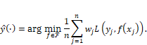
Equation 9.1

(Compare this to Equation 7.3, which is the same thing, but without the weights.) The importance weight is the ratio of the probability density of the features  under the deployment distribution and the training distribution: .[9] The weighting scheme tries to make the African features look more like the Indian features by emphasizing those that are less likely in East and Central African countries but more likely in India.

How do you compute the weight from the training and deployment datasets? You could first try to estimate the two pdfs separately and then evaluate them at each training data point and plug them into the ratio. But that usually doesn’t work well. The better way to go is to directly estimate the weight.

“When solving a problem of interest, do not solve a more general problem as an intermediate step.”

—Vladimir Vapnik, computer scientist at AT&T Bell Labs

The most straightforward technique is similar to computing propensity scores in Chapter 8. You learn a classifier with a calibrated continuous score  such as logistic regression or any other classifier from Chapter 7. The dataset to train this classifier is a concatenation of the deployment and training datasets. The labels are  for the data points that come from the deployment dataset and the labels are  for the data points that come from the training dataset. The features are the features. Once you have the continuous output of the classifier as a score, the importance weight is:[10]

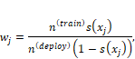
Equation 9.2

where  and  are the number of data points in the training and deployment datasets, respectively.

9.3.3        Concept Drift

Adapting to prior probability shift and covariate shift can be done without labels from the deployment data because they come from sampling bias in which the relationship between features and labels does not change. However, the same thing is not possible under concept drift because it comes from measurement bias: the relationship between features and labels changing from African countries to India. To adapt to concept drift, you must be very judicious in selecting unlabeled deployment data points to (expensively) get labels for. It could mean having a human expert in India look at some applications and provide judgement on whether to approve or deny the mobile money-enabled credit. There are various criteria for choosing points for such annotation. Once you’ve gotten the annotations, retrain the classifier on the newly labeled data from India (possibly with large weight) along with the older training data from East and Central African countries (possibly with small weight).

 

9.4           Robustness

Often, you do not have any data from the deployment environment, so adaptation is out of the question. You might not even know what the deployment environment is going to be. It might not even end up being India for all that you know. Robustness does not require you to have any deployment data. It modifies the learning objective and procedure.

9.4.1        Prior Probability Shift

If you don’t have any data from the deployment environment (India), you want to make your model robust to whatever prior probabilities of creditworthiness there could be. Consider a situation in which the deployment prior probabilities in India are actually  and , but you guess that they are  and , maybe by looking at the prior probabilities in the different African countries. Your guess is probably a little bit off. If you use the decision function corresponding to your guess with the likelihood ratio test threshold  (recall this was the form of the optimal threshold stated in Chapter 6), it has the following mismatched Bayes risk performance:[11]

Equation 9.3

You lose out on performance. Your epistemic uncertainty in knowing the right prior probabilities has hurt the Bayes risk.

To be robust to the uncertain prior probabilities in present-day India, choose a value for  so that the worst-case performance is as good as possible. Known as a min-max formulation, the problem is to find a min-max optimal prior probability point that you’re going to use when you deploy the Phulo model. Specifically, you want:

Equation 9.4

Normally in the book, we stop at the posing of the formulation. In this instance, however, since the min-max optimal solution has nice geometric properties, let’s carry on. The mismatched Bayes risk function  is a linear function of  for a fixed value of . When , the Bayes optimal threshold is recovered and  is the optimal Bayes risk  defined in Chapter 6. It is a concave function that is zero at the endpoints of the interval .[12] The linear mismatched Bayes risk function is tangent to the optimal Bayes risk function at  and greater than it everywhere else.[13] This relationship is shown in Figure 9.6.

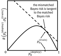
Figure 9.6. An example mismatched (dashed line) and matched Bayes risk function (solid curve). Accessible caption. A plot with  on the vertical axis and  on the horizontal axis. The matched Bayes risk is 0 at , increases to a peak in the middle and decreases back to 0 at . Its shape is concave. The mismatched Bayes risk is a line tangent to the matched Bayes risk at the point , which in this example is at a point greater than the peak of the matched Bayes risk. There’s a large gap between the matched and mismatched Bayes risk, especially towards .

The solution is the prior probability value at which the matched Bayes risk function has zero slope. It turns out that the correct answer is the place where the mismatched Bayes risk tangent line is flat—at the top of the hump as shown in Figure 9.7. Once you have it, use it in the threshold of the Phulo decision function to deal with prior probability shift.

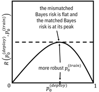
Figure 9.7. The most robust prior probability to use in the decision function place is where the matched Bayes risk function is maximum. Accessible caption. A plot with  on the vertical axis and  on the horizontal axis. The matched Bayes risk is 0 at , increases to a peak in the middle and decreases back to 0 at . Its shape is concave. The mismatched Bayes risk is a horizontal line tangent to the matched Bayes risk at the optimal point , which is at the peak of the matched Bayes risk. The maximum gap between the matched and mismatched Bayes risk is as small as can be.

9.4.2        Covariate Shift

If you are in the covariate shift setting instead of being in the prior probability shift setting, you have to do something a little differently to make your model robust to the deployment environment. Here too, robustness means setting up a min-max optimization problem so that you do the best that you can in preventing the worst-case behavior. Starting from the importance weight formulation of Equation 9.1, put in an extra maximum loss over the weights:[14]

Equation 9.5

where  is the set of possible weights that are non-negative and sum to one. The classifier that optimizes the objective in Equation 9.5 is the robust classifier you’ll want to use for the Phulo model to deal with covariate shift.

9.4.3        Concept Drift and Other Distribution Shifts

Just like adapting to concept drift is harder than adapting to prior probability shift and covariate shift because it stems from measurement bias instead of sampling bias, robustness to concept drift is also harder. It is one of the most vexing problems in machine learning. You can’t really pose a min-max formulation because the training data from East and Central African countries is not indicating the right relationship between the features and label in India. A model robust to concept drift must extrapolate outside of what the training data can tell you. And that is too open-ended of a task to do well unless you make some more assumptions.

One reasonable assumption you can make is that the set of features split into two types: (1) causal or stable features, and (2) spurious features. You don’t know which ones are which beforehand. The causal features capture the intrinsic parts of the relationship between features and labels, and are the same set of features in different environments. In other words, this set of features is invariant across the environments. Spurious features might be predictive in one environment or a few environments, but not universally so across environments. You want the Phulo model to rely on the causal features whose predictive relationship with labels holds across Tanzania, Rwanda, Congo, and all the other countries that Wavetel has data from and ignore the spurious features. By doing so, the hope is that the model will not only perform well for the countries in the training set, but also any new country or environment that it encounters, such as India. It will be robust to the environment in which it is deployed.

“ML enables an increased emphasis on stability and robustness.”

—Susan Athey, economist at Stanford University

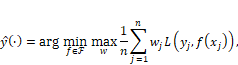
Invariant risk minimization is a variation on the standard risk minimization formulation of machine learning that helps the model focus on the causal features and avoid the spurious features when there is data from more than one environment available for training. The formulation is:[15]

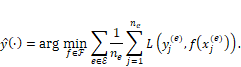
Equation 9.6

Let’s break this equation down bit by bit to understand it more. First, the set  is the set of all environments or countries from which we have training data (Tanzania, Rwanda, Congo, etc.) and each country is indexed by . There are  training samples  from each country. The inner summation in the top line is the regular risk expression that we’ve seen before in Chapter 7. 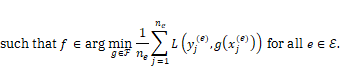The outer summation in the top line is just adding up all the risks for all the environments, so that the classifier minimizes the total risk. The interesting part is the constraint in the second line. It is saying that the classifier that is the solution of the top line must simultaneously minimize the risk for each of the environments or countries separately as well. As you know from earlier in the chapter, there can be many different classifiers that minimize the loss—they are the Rashomon set—and that is why the second line has the ‘element of’ symbol . The invariant risk minimization formulation adds extra specification to reduce the epistemic uncertainty and allow for better out-of-distribution generalization.

You might ask yourself whether the constraint in the second line does anything useful. Shouldn’t the first line alone give you the same solution? This is a question that machine learning researchers are currently struggling with.[16] They find that usually, the standard risk minimization formulation of machine learning from Chapter 7 is the most robust to general distribution shifts, without the extra invariant risk minimization constraints. However, when the problem is an anticausal learning problem and the feature distributions across environments have similar support, invariant risk minimization may outperform standard machine learning (remember from earlier in the chapter that the label causes the features in anticausal learning).[17]

In a mobile money-enabled credit approval setting like you have with Phulo, it is not entirely clear whether the problem is causal learning or anticausal learning: do the features cause the label or do the labels cause the features? In a traditional credit scoring problem, you are probably in the causal setting because there are strict parameters on features like salary and assets that cause a person to be viewed by a bank as creditworthy or not. In the mobile money and unbanked setting, you could also imagine the problem to be anticausal if you think that a person is inherently creditworthy or not, and the features you’re able to collect from their mobile phone usage are a result of the creditworthiness. As you’re developing the Phulo model, you should give invariant risk minimization a shot because you have datasets from several countries, require robustness to concept drift and generalization to new countries, and likely have an anticausal learning problem. You and your data science team can be happy that you’ve given Wavetel and the Bank of Bulandshahr a model they can rely on during the launch of Phulo.

 

9.5           Summary

§  Machine learning models should not take shortcuts if they are to be reliable. You must minimize epistemic uncertainty in modeling, data preparation, sampling, and measurement.

§  Data augmentation is a way to reduce epistemic uncertainty in modeling.

§  Distribution shift—the mismatch between the probability distribution of the training data and the data you will see during deployment—has three special cases: prior probability shift, covariate shift, and concept drift. Often, you can’t detect distribution shift. You just have to assume it.

§  Prior probability shift and covariate shift are easier to overcome than concept drift because they arise from sampling bias rather than measurement bias.

§  A pre-processing strategy for mitigating prior probability shift and covariate shift is adaptation, in which sample weights multiply the training loss during the model learning process. Finding the weights requires a fixed target deployment distribution and unlabeled data from it.

§  A strategy for mitigating prior probability and covariate shift during model training is min-max robustness, which changes the learning formulation to try to do the best in the worst-case environment that could be encountered during deployment.

§  Adapting to concept drift requires the acquisition of some labeled data from the deployment environment.

§  Invariant risk minimization is a strategy for mitigating concept drift and achieving distributional robustness that focuses the model’s efforts on causal features and ignores spurious features. It may work well in anticausal learning scenarios in which the label causes the features.