6
Detection Theory
Let’s continue from Chapter 3, where you are the data scientist building the loan approval model for the (fictional) peer-to-peer lender ThriveGuild. As then, you are in the first stage of the machine learning lifecycle, working with the problem owner to specify the goals and indicators of the system. You have already clarified that safety is important, and that it is composed of two parts: basic performance (minimizing aleatoric uncertainty) and reliability (minimizing epistemic uncertainty). Now you want to go into greater depth in the problem specification for the first part: basic performance. (Reliability comes in Part 4 of the book.)
What are the different quantitative metrics you could use in translating the problem-specific goals (e.g. expected profit for the peer-to-peer lender) to machine learning quantities? Once you’ve reached the modeling stage of the lifecycle, how would you know you have a good model? Do you have any special considerations when producing a model for risk assessment rather than simply offering an approve/deny output?
Machine learning models are decision functions: based on the borrower’s features, they decide a response that may lead to an autonomous approval/denial action or be used to support the decision making of the loan officer. The use of decision functions is known as statistical discrimination because we are distinguishing or differentiating one class label from the other. You should contrast the use of the term ‘discrimination’ here with unwanted discrimination that leads to systematic advantages to certain groups in the context of algorithmic fairness in Chapter 10. Discrimination here is simply telling the difference between things. Your favorite wine snob talking about their discriminative palate is a distinct concept from racial discrimination.
This chapter begins Part 3 of the book on basic modeling (see Figure 6.1 to remind yourself of the lay of the land) and uses detection theory, the study of optimal decision making in the case of categorical output responses,[1] to answer the questions above that you are struggling with.
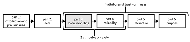
Figure 6.1. Organization of the book. This third part focuses on the first attribute of trustworthiness, competence and credibility, which maps to machine learning models that are well-performing and accurate. Accessible caption. A flow diagram from left to right with six boxes: part 1: introduction and preliminaries; part 2: data; part 3: basic modeling; part 4: reliability; part 5: interaction; part 6: purpose. Part 3 is highlighted. Parts 3–4 are labeled as attributes of safety. Parts 3–6 are labeled as attributes of trustworthiness.
Specifically, this chapter focuses on:
§ selecting metrics to quantify the basic performance of your decision function (including ones that summarize performance across operating conditions),
§ testing whether your decision function is as good as it could ever be, and
§ differentiating performance in risk assessment problems from performance in binary decision problems.
6.1 Selecting Decision Function Metrics
You,
the ThriveGuild data scientist, are faced with the binary
detection problem, also known as the binary hypothesis testing problem, of predicting which
loan applicants will default, and thereby which applications to deny.[2]
Let ![]() be the loan
approval decision with label
be the loan
approval decision with label ![]() corresponding to
corresponding to ![]() and label
and label ![]() corresponding to
corresponding to ![]() . Feature vector
. Feature vector ![]() contains
employment status, income, and other attributes. The value
contains
employment status, income, and other attributes. The value ![]() is called a negative and the value
is called a negative and the value ![]() is called a positive. The random variables for the features and label
are governed by the pmfs given the special name likelihood
functions
is called a positive. The random variables for the features and label
are governed by the pmfs given the special name likelihood
functions ![]() and
and ![]() , as well as by prior probabilities
, as well as by prior probabilities ![]() and
and ![]() . The basic task is
to find a decision function
. The basic task is
to find a decision function ![]() that predicts a
label from the features.[3]
that predicts a
label from the features.[3]
6.1.1 Quantifying the Possible Events
There are four possible events in the binary detection problem:
1.
the
decision function predicts ![]() and the true label
is
and the true label
is ![]() ,
,
2.
the
decision function predicts ![]() and the true label
is
and the true label
is ![]() ,
,
3.
the
decision function predicts ![]() and the true label
is
and the true label
is ![]() , and
, and
4.
the
decision function predicts ![]() and the true label
is
and the true label
is ![]() .
.
These are known as true negatives (TN), false negatives (FN), true positives (TP), and false positives (FP), respectively. A true negative is denying an applicant who should be denied according to some ground truth, a false negative is denying an applicant who should be approved, a true positive is approving an applicant who should be approved, and a false positive is approving an applicant who should be denied. Let’s organize these events in a table known as the confusion matrix:
|
|
|
|
|
|
|
|
|
|
|
|
Equation 6.1
The probabilities of these events are:
|
|
|
|
|
|
Equation 6.2
These
conditional probabilities are nothing more than a direct implementation of the
definitions of the events. The probability ![]() is known as the true negative rate as well as the specificity and the
selectivity. The probability
is known as the true negative rate as well as the specificity and the
selectivity. The probability ![]() is known as the false negative rate as well as the probability of missed
detection and the miss rate. The probability
is known as the false negative rate as well as the probability of missed
detection and the miss rate. The probability ![]() is known as the true positive rate as well as the probability of
detection, the recall, the sensitivity, and the power. The probability
is known as the true positive rate as well as the probability of
detection, the recall, the sensitivity, and the power. The probability ![]() is known as the false positive rate as well as the probability of false
alarm and the fall-out. The probabilities can be organized in a slightly
different table as well:
is known as the false positive rate as well as the probability of false
alarm and the fall-out. The probabilities can be organized in a slightly
different table as well:
|
|
|
|
|
|
|
|
|
|
|
|
Equation 6.3
These
probabilities give you some quantities by which to understand the performance
of the decision function ![]() . Selecting one
over the other involves thinking about the events themselves and how they
relate to the real-world problem. A false positive, approving an applicant who
should be denied, means that a ThriveGuild lender has to bear the cost of a
default, so it should be kept small. A false negative, denying an applicant who
should be approved, is a lost opportunity for ThriveGuild to make a profit through
the interest they charge.
. Selecting one
over the other involves thinking about the events themselves and how they
relate to the real-world problem. A false positive, approving an applicant who
should be denied, means that a ThriveGuild lender has to bear the cost of a
default, so it should be kept small. A false negative, denying an applicant who
should be approved, is a lost opportunity for ThriveGuild to make a profit through
the interest they charge.
The events above are conditioned on the true label. Conditioning on the predicted label also yields events and probabilities of interest in characterizing performance:
|
|
|
|
|
|
|
|
|
|
|
|
Equation 6.4
These
conditional probabilities are reversed from Equation 6.2. The probability ![]() is known as the negative predictive value. The probability
is known as the negative predictive value. The probability ![]() is known as the false omission rate. The probability
is known as the false omission rate. The probability ![]() is known as the positive predictive value as well as the precision. The
probability
is known as the positive predictive value as well as the precision. The
probability ![]() is known as the false discovery rate. If you care about the quality of the
decision function, focus on the first set (
is known as the false discovery rate. If you care about the quality of the
decision function, focus on the first set (![]() ,
, ![]() ,
, ![]() ,
, ![]() ). If you care
about the quality of the predictions, focus on the second set (
). If you care
about the quality of the predictions, focus on the second set (![]() ,
, ![]() ,
, ![]() ,
, ![]() ).
).
When
you need to numerically compute these probabilities, apply the decision
function to several i.i.d. samples of ![]() and denote the
number of TN, FN, TP, and FP events as
and denote the
number of TN, FN, TP, and FP events as ![]() ,
, ![]() ,
, ![]() , and
, and ![]() , respectively. Then
use the following estimates of the probabilities:
, respectively. Then
use the following estimates of the probabilities:
|
|
|
|
|
|
|
|
|
|
|
|
Equation 6.5
As
an example, let’s say that ThriveGuild makes the following number of decisions:
![]() ,
, ![]() ,
, ![]() , and
, and ![]() . You can estimate
the various performance probabilities by plugging these numbers into the
respective expressions above. The results are
. You can estimate
the various performance probabilities by plugging these numbers into the
respective expressions above. The results are ![]() ,
, ![]() ,
, ![]() ,
, ![]() ,
, ![]() ,
, ![]() ,
, ![]() , and
, and ![]() . These are all
reasonably good values, but must ultimately be judged according to the ThriveGuild
problem owner's goals and objectives.
. These are all
reasonably good values, but must ultimately be judged according to the ThriveGuild
problem owner's goals and objectives.
6.1.2 Summary Performance Metrics
Collectively, false negatives and false positives are errors. The probability of error, also known as the error rate, is the sum of the false negative rate and false positive rate weighted by the prior probabilities:
![]()
Equation 6.6
The balanced probability of error, also known as the balanced error rate, is the unweighted average of the false negative rate and false positive rate:
![]()
Equation 6.7
They
summarize the basic performance of the decision function. Balancing is useful
when there are a lot more data points with one label than the other, and you
care about each type of error equally. Accuracy, the
complement of the probability of error: ![]() , and balanced accuracy, the complement of the balanced probability
of error:
, and balanced accuracy, the complement of the balanced probability
of error: ![]() , are sometimes
easier for problem owners to appreciate than error rates.
, are sometimes
easier for problem owners to appreciate than error rates.
The
![]() -score, the
harmonic mean of
-score, the
harmonic mean of ![]() and
and ![]() , is an
accuracy-like summary measure to characterize the quality of a prediction
rather than the decision function:
, is an
accuracy-like summary measure to characterize the quality of a prediction
rather than the decision function:
![]()
Equation 6.8
Continuing
the example from before with ![]() and
and ![]() , let ThriveGuild’s
prior probability of receiving applications to be denied according to some
ground truth be
, let ThriveGuild’s
prior probability of receiving applications to be denied according to some
ground truth be ![]() and applications
to be approved be
and applications
to be approved be ![]() . Then, plugging in
to the relevant equations above, you’ll find ThriveGuild to have
. Then, plugging in
to the relevant equations above, you’ll find ThriveGuild to have ![]() ,
, ![]() , and
, and ![]() . Again, these are
reasonable values that may be deemed acceptable to the problem owner.
. Again, these are
reasonable values that may be deemed acceptable to the problem owner.
As
the data scientist, you can get pretty far with these abstract TN, FN, TP, and
FP events, but they have to be put in the context of the problem owner’s goals.
ThriveGuild cares about making good bets on borrowers so that they are
profitable. More generally across real-world applications, error events yield
significant consequences to affected people including loss of life, loss of
liberty, loss of livelihood, etc. Therefore, to truly characterize the
performance of a decision function, it is important to consider the costs associated with the different events. You can
capture these costs through a cost function ![]() and denote the
costs as
and denote the
costs as ![]() ,
, ![]() ,
, ![]() , and
, and ![]() , respectively.
, respectively.
Taking
costs into account, the characterization of performance for the decision
function is known as the Bayes risk ![]() :
:
![]()
Equation 6.9
Breaking
the equation down, you’ll see that the two error probabilities, ![]() and
and ![]() are the main
components, multiplied by their relevant prior probabilities and costs. The
costs of the non-error events appear just multiplied by their costs. The Bayes
risk is the performance metric most often used in finding optimal decision
functions. Actually finding the decision function is known as solving the Bayesian detection problem. Eliciting the cost function
are the main
components, multiplied by their relevant prior probabilities and costs. The
costs of the non-error events appear just multiplied by their costs. The Bayes
risk is the performance metric most often used in finding optimal decision
functions. Actually finding the decision function is known as solving the Bayesian detection problem. Eliciting the cost function ![]() for a given
real-world problem from the problem owner is part of value alignment, described
in Chapter 14.
for a given
real-world problem from the problem owner is part of value alignment, described
in Chapter 14.
A mental model or roadmap, shown in Figure 6.2, to hold throughout the rest of the chapter is that the Bayes risk and the Bayesian detection problem are the central concept, and all other concepts are related to the central concept in various ways and for various purposes. The terms and concepts that have not yet been defined and evaluated are coming up soon.
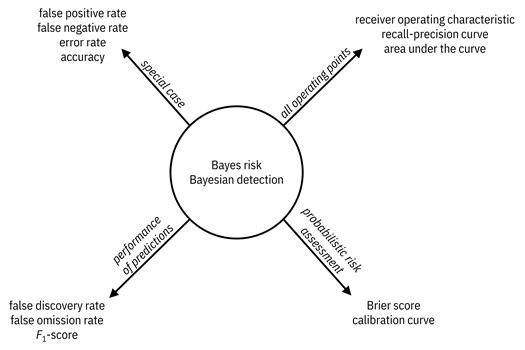
Figure 6.2. A mental model for different concepts in
detection theory surrounding the central concept of Bayes risk and Bayesian
detection. A diagram with Bayes risk and Bayesian detection at the center
and four other groups of concepts radiating outwards. False positive rate,
false negative rate, error rate, and accuracy are special cases. Receiver
operating characteristic, recall-precision curve, and area under the curve
arise when examining all operating points. Brier score and calibration curve
arise in probabilistic risk assessment. False discover rate, false omission
rate, and ![]() -score relate to
performance of predictions.
-score relate to
performance of predictions.
Because
getting things right is a good thing, it is often assumed that there is no cost
to correct decisions, i.e., ![]() and
and ![]() , which is also
assumed in this book going forward. In this case, the Bayes risk simplifies to:
, which is also
assumed in this book going forward. In this case, the Bayes risk simplifies to:
![]()
Equation 6.10
To
arrive at this simplified equation, just insert zeros for ![]() and
and ![]() in Equation 6.9. The
Bayes risk with
in Equation 6.9. The
Bayes risk with ![]() and
and ![]() is the probability
of error.
is the probability
of error.
We
are implicitly assuming that ![]() does not depend on
does not depend on
![]() except through
except through ![]() . This assumption
is not required, but made for simplicity. You can easily imagine scenarios in
which the cost of a decision depends on the feature. For example, if one of the
features used in the loan approval decision by ThriveGuild is the value of the
loan, the cost of an error (monetary loss) depends on that feature.
Nevertheless, for simplicity, we usually make the assumption that the cost
function does not explicitly depend on the feature value. For example, under
this assumption, the cost of a false negative may be
. This assumption
is not required, but made for simplicity. You can easily imagine scenarios in
which the cost of a decision depends on the feature. For example, if one of the
features used in the loan approval decision by ThriveGuild is the value of the
loan, the cost of an error (monetary loss) depends on that feature.
Nevertheless, for simplicity, we usually make the assumption that the cost
function does not explicitly depend on the feature value. For example, under
this assumption, the cost of a false negative may be ![]() and the cost of a
false positive
and the cost of a
false positive ![]() for all applicants.
for all applicants.
6.1.3 Accounting for Different Operating Points
The
Bayes risk is all well and good if there is a fixed set of prior probabilities
and a fixed set of costs, but things change. If the economy improves, potential
borrowers might become more reliable in loan repayment. If a different problem
owner comes in and has a different interpretation of opportunity cost, then the
cost of false negatives ![]() changes. How
should you think about the performance of decision functions across different
sets of those values, known as different operating points?
changes. How
should you think about the performance of decision functions across different
sets of those values, known as different operating points?
Many
decision functions are parameterized by a threshold ![]() (including the
optimal decision function that will be demonstrated in Section 6.2). You can
change the decision function to be more or less forgiving of false positives or
false negatives, but not both at the same time. Varying
(including the
optimal decision function that will be demonstrated in Section 6.2). You can
change the decision function to be more or less forgiving of false positives or
false negatives, but not both at the same time. Varying ![]() explores this
tradeoff and yields different error probability pairs
explores this
tradeoff and yields different error probability pairs ![]() , i.e. different
operating points. Equivalently, different operating points correspond to
different false positive rate and true positive rate pairs
, i.e. different
operating points. Equivalently, different operating points correspond to
different false positive rate and true positive rate pairs ![]() . The curve traced
out on the
. The curve traced
out on the ![]() –
–![]() plane as the parameter
plane as the parameter
![]() is varied from
zero to infinity is the receiver operating characteristic
(ROC). The ROC takes values
is varied from
zero to infinity is the receiver operating characteristic
(ROC). The ROC takes values ![]() when
when ![]() and
and ![]() when
when ![]() . You can
understand this because at one extreme, the decision function always says
. You can
understand this because at one extreme, the decision function always says ![]() ; in this case
there are no FPs and no TPs. At the other extreme, the decision function always
says
; in this case
there are no FPs and no TPs. At the other extreme, the decision function always
says ![]() ; in this case all
decisions are either FPs or TPs.
; in this case all
decisions are either FPs or TPs.
The
ROC is a concave, nondecreasing function illustrated in Figure 6.3. The closer
to the top left corner it goes, the better. The best ROC for discrimination
goes straight up to ![]() and then makes a
sharp turn to the right. The worst ROC is the diagonal line connecting
and then makes a
sharp turn to the right. The worst ROC is the diagonal line connecting ![]() and
and ![]() achieved by random
guessing. The area under the ROC, also known as the area
under the curve (AUC) synthesizes performance across all operating
points and should be selected as a metric when it is likely that the same
threshold-parameterized decision function will be applied in very different
operating conditions. Given the shapes of the worst (diagonal line) and best
(straight up and then straight to the right) ROC curves, you can see that the
AUC ranges from
achieved by random
guessing. The area under the ROC, also known as the area
under the curve (AUC) synthesizes performance across all operating
points and should be selected as a metric when it is likely that the same
threshold-parameterized decision function will be applied in very different
operating conditions. Given the shapes of the worst (diagonal line) and best
(straight up and then straight to the right) ROC curves, you can see that the
AUC ranges from ![]() (area of bottom
right triangle) to
(area of bottom
right triangle) to ![]() (area of entire
square).[4]
(area of entire
square).[4]
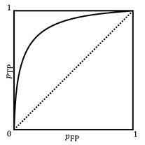
Figure 6.3. An example receiver operating characteristic
(ROC). Accessible caption. A plot with ![]() on the vertical
axis and
on the vertical
axis and ![]() on the horizontal
axis. Both axes range from
on the horizontal
axis. Both axes range from ![]() to
to ![]() . A dashed diagonal
line goes from
. A dashed diagonal
line goes from ![]() to
to ![]() and corresponds to
random guessing. A solid concave curve, the ROC, goes from
and corresponds to
random guessing. A solid concave curve, the ROC, goes from ![]() to
to ![]() staying above and
to the left of the diagonal line.
staying above and
to the left of the diagonal line.
6.2 The Best That You Can Ever Do
As the ThriveGuild data scientist, you have given the problem owner an entire menu of basic performance measures to select from and indicated when different choices are more and less appropriate. The Bayes risk is the most encompassing and most often used performance characterization for a decision function. Let’s say that Bayes risk was chosen in the problem specification stage of the machine learning lifecycle, including selecting the costs. Now you are in the modeling stage and need to figure out if the model is performing well. The best way to do that is to optimize the Bayes risk to obtain the best possible decision function with the smallest Bayes risk and compare the current model’s Bayes risk to it.
“The predictability ceiling is often ignored in mainstream ML research. Every prediction problem has an upper bound for prediction—the Bayes-optimal performance. If you don't have a good sense of what it is for your problem, you are in the dark.”
—Mert R. Sabuncu, computer scientist at Cornell University
Let
us denote the best possible decision function as ![]() and its
corresponding Bayes risk as
and its
corresponding Bayes risk as ![]() . They are
specified using the minimization of the expected cost:
. They are
specified using the minimization of the expected cost:
![]()
Equation 6.11
where
the expectation is over both ![]() and
and ![]() . Because it
achieves the minimal cost, the function
. Because it
achieves the minimal cost, the function ![]() is the best
possible
is the best
possible ![]() by definition.
Whatever Bayes risk
by definition.
Whatever Bayes risk ![]() it has, no other
decision function can have a lower Bayes risk
it has, no other
decision function can have a lower Bayes risk ![]() .
.
We aren’t going to work it out here, but the solution to the minimization problem in Equation 6.11 is the Bayes optimal decision function, and takes the following form:
![]()
Equation 6.12
where
![]() , known as the likelihood ratio, is defined as:
, known as the likelihood ratio, is defined as:
![]()
Equation 6.13
and
![]() , known as the threshold, is defined as:
, known as the threshold, is defined as:
![]()
Equation 6.14
The
likelihood ratio is as its name says: it is the ratio of the likelihood
functions. It is a scalar value even if the features ![]() are multivariate. As
the ratio of two non-negative pdf values, it has the range
are multivariate. As
the ratio of two non-negative pdf values, it has the range ![]() and can be viewed
as a random variable. The threshold is made up of both costs and prior
probabilities. This optimal decision function
and can be viewed
as a random variable. The threshold is made up of both costs and prior
probabilities. This optimal decision function ![]() given in Equation 6.12
is known as the likelihood ratio test.
given in Equation 6.12
is known as the likelihood ratio test.
6.2.1 Example
As
an example, let ThriveGuild’s loan approval decision be determined solely by
one feature ![]() : the income of the
applicant. Recall that we modeled income to be exponentially-distributed in Chapter
3. Specifically, let
: the income of the
applicant. Recall that we modeled income to be exponentially-distributed in Chapter
3. Specifically, let ![]() and
and ![]() , both for
, both for ![]() . Like earlier in
this chapter,
. Like earlier in
this chapter, ![]() ,
, ![]() ,
, ![]() , and
, and ![]() . Then simply
plugging in to Equation 6.13, you’ll get:
. Then simply
plugging in to Equation 6.13, you’ll get:
![]()
Equation 6.15
and plugging in to Equation 6.14, you’ll get:
![]()
Equation 6.16
Plugging these expressions into the Bayes optimal decision function given in Equation 6.12, you’ll get:
![]()
Equation 6.17
which can be simplified to:
![]()
Equation 6.18
by
multiplying both sides of the inequalities in both cases by ![]() , taking the
natural logarithm, and then multiplying by
, taking the
natural logarithm, and then multiplying by ![]() again. Applicants
with an income less than or equal to
again. Applicants
with an income less than or equal to ![]() are denied and
applicants with an income greater than
are denied and
applicants with an income greater than ![]() are approved. The
expected value of
are approved. The
expected value of ![]() is
is ![]() and the expected
value of
and the expected
value of ![]() is
is ![]() . Thus in this
example, an applicant's income has to be quite a bit higher than the mean to be
approved.
. Thus in this
example, an applicant's income has to be quite a bit higher than the mean to be
approved.
You
should use the Bayes-optimal risk ![]() to lower bound the
performance of any machine learning classifier that you might try for a given
data distribution.[5]
No matter how hard you work or how creative you are, you can never overcome the
Bayes limit. So you should be happy if you get close. If the Bayes-optimal risk
itself is too high, then the thing to do is to go back to the data understanding
and data preparation stages of the machine learning lifecycle and get more
informative data.
to lower bound the
performance of any machine learning classifier that you might try for a given
data distribution.[5]
No matter how hard you work or how creative you are, you can never overcome the
Bayes limit. So you should be happy if you get close. If the Bayes-optimal risk
itself is too high, then the thing to do is to go back to the data understanding
and data preparation stages of the machine learning lifecycle and get more
informative data.
6.3 Risk Assessment and Calibration
To approve or to deny, that is the question for ThriveGuild. Or is it? Maybe the question is actually: what is the probability that the borrower will default? Maybe the problem is not binary classification, but probabilistic risk assessment. It is certainly an option for you, the data scientist, and the problem owner to consider during problem specification. Thresholding a probabilistic risk assessment yields a classification, but there are a few subtleties for you to weigh.
The
likelihood ratio ranges from zero to infinity and the threshold value ![]() is optimal for
equal priors and equal costs. Applying any monotonically increasing function to
both the likelihood ratio and the threshold still yields a Bayes optimal
decision function with the same risk
is optimal for
equal priors and equal costs. Applying any monotonically increasing function to
both the likelihood ratio and the threshold still yields a Bayes optimal
decision function with the same risk ![]() . That is,
. That is,
![]()
Equation 6.19
for
any monotonically increasing function ![]() is still optimal.
is still optimal.
It
is somewhat more natural to think of a score ![]() to be in the range
to be in the range
![]() because it
corresponds to the label values
because it
corresponds to the label values ![]() and could also
potentially be interpreted as a probability. The score, a continuous-valued
output of the decision function, can then be thought of as a confidence in the
prediction and be obtained by applying a suitable
and could also
potentially be interpreted as a probability. The score, a continuous-valued
output of the decision function, can then be thought of as a confidence in the
prediction and be obtained by applying a suitable ![]() function to the
likelihood ratio. In this case,
function to the
likelihood ratio. In this case, ![]() is the threshold
for equal priors and costs. Intermediate score values are less confident and
extreme score values (towards
is the threshold
for equal priors and costs. Intermediate score values are less confident and
extreme score values (towards ![]() and
and ![]() ) are more
confident. Just as the likelihood ratio may be viewed as a random variable, the
score may also be viewed as a random variable
) are more
confident. Just as the likelihood ratio may be viewed as a random variable, the
score may also be viewed as a random variable ![]() . The Brier score is an appropriate performance metric for the
continuous-valued output score of the decision function:
. The Brier score is an appropriate performance metric for the
continuous-valued output score of the decision function:
![]()
Equation 6.20
It
is the mean-squared error of the score ![]() with respect to
the true label
with respect to
the true label ![]() . For a finite
number of samples
. For a finite
number of samples ![]() , you can compute
it as:
, you can compute
it as:
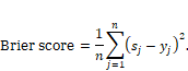
Equation 6.21
The
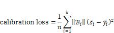
Brier score decomposes into the sum of two separable components: calibration and refinement.[6]
The concept of calibration is that the predicted score corresponds to the
proportion of positive true labels. For example, a bunch of data points all
having a calibrated score of ![]() implies that 70%
of them have true label
implies that 70%
of them have true label ![]() and 30% of them
have true label
and 30% of them
have true label ![]() . Said another way,
perfect calibration implies that the probability of the true label
. Said another way,
perfect calibration implies that the probability of the true label ![]() being
being ![]() given the
predicted score
given the
predicted score ![]() being
being ![]() is the value
is the value ![]() itself:
itself: ![]() Calibration is
important for probabilistic risk assessments: a perfectly calibrated score can
be interpreted as a probability of predicting one class or the other. It is
also an important concept for evaluating causal inference methods, described in
Chapter 8, for algorithmic fairness, described in Chapter 10, and for
communicating uncertainty, described in Chapter 13.
Calibration is
important for probabilistic risk assessments: a perfectly calibrated score can
be interpreted as a probability of predicting one class or the other. It is
also an important concept for evaluating causal inference methods, described in
Chapter 8, for algorithmic fairness, described in Chapter 10, and for
communicating uncertainty, described in Chapter 13.
Since
any monotonically increasing transformation ![]() can be applied to
a decision function without changing its ability to discriminate, you can
improve the calibration of a decision function by finding a better
can be applied to
a decision function without changing its ability to discriminate, you can
improve the calibration of a decision function by finding a better ![]() . The calibration
loss quantitatively captures how close a decision function is to perfect calibration.
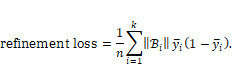
The refinement loss is a sort of variance of how tightly the true labels
distribute around a given score. For
. The calibration
loss quantitatively captures how close a decision function is to perfect calibration.
The refinement loss is a sort of variance of how tightly the true labels
distribute around a given score. For ![]() that have been
sorted by their score values and binned into
that have been
sorted by their score values and binned into ![]() groups
groups ![]() with average
values
with average
values ![]() within the bins
within the bins
Equation 6.22
As stated earlier, the sum of the calibration loss and refinement loss is the Brier score.
A
calibration curve, also known as a reliability
diagram, shows the ![]() values as a plot.
One example is shown in Figure 6.4. The closer to a straight diagonal from
values as a plot.
One example is shown in Figure 6.4. The closer to a straight diagonal from ![]() to
to ![]() , the better.
Plotting this curve is a good diagnostic tool for you to understand the
calibration of a decision function.
, the better.
Plotting this curve is a good diagnostic tool for you to understand the
calibration of a decision function.
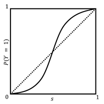
Figure 6.4. An example calibration curve. Accessible
caption. A plot with![]() on the vertical
axis and
on the vertical
axis and ![]() on the horizontal
axis. Both axes range from
on the horizontal
axis. Both axes range from ![]() to
to ![]() . A dashed diagonal
line goes from
. A dashed diagonal
line goes from ![]() to
to ![]() and corresponds to
perfect calibration. A solid S-shaped curve, the calibration curve, goes from
and corresponds to
perfect calibration. A solid S-shaped curve, the calibration curve, goes from ![]() to
to ![]() starting below and
to the right of the diagonal line before crossing over to being above and to
the left of the diagonal line.
starting below and
to the right of the diagonal line before crossing over to being above and to
the left of the diagonal line.
6.4 Summary
§ Four possible events result from binary decisions: false negatives, true negatives, false positives, and true positives.
§ Different ways to combine the probabilities of these events lead to classifier performance metrics appropriate for different real-world contexts.
§ One important one is Bayes risk: the combination of the false negative probability and false positive probability weighted by both the costs of those errors and the prior probabilities of the labels. It is the basic basic performance measure for the first attribute of safety and trustworthiness.
§ Detection theory, the study of optimal decisions, which provides fundamental limits to how well machine learning models may ever perform is a tool for you to assess the basic performance of your models.
§ Decision functions may output continuous-valued scores rather than only hard, zero or one, decisions. Scores indicate confidence in a prediction. Calibrated scores are those for which the score value is the probability of a sample belonging to a label class.