1    

2    

3    

Safety

Imagine that you are a data scientist at the (fictional) peer-to-peer lender ThriveGuild. You are in the problem specification phase of the machine learning lifecycle for a system that evaluates and approves borrowers. The problem owners, diverse stakeholders, and you yourself want this system to be trustworthy and not cause harm to people. Everyone wants it to be safe. But what is harm and what is safety in the context of a machine learning system?

Safety can be defined in very domain-specific ways, like safe toys not having lead paint or small parts that pose choking hazards, safe neighborhoods having low rates of violent crime, and safe roads having a maximum curvature. But these definitions are not particularly useful in helping define safety for machine learning. Is there an even more basic definition of safety that could be extended to the machine learning context? Yes, based on the concepts of (1) harm, (2) aleatoric uncertainty and risk, and (3) epistemic uncertainty.[1] (These terms are defined in the next section.)

This chapter teaches you how to approach the problem specification phase of a trustworthy machine learning system from a safety perspective. Specifically, by defining safety as minimizing two different types of uncertainty, you can collaborate with problem owners to crisply specify safety requirements and objectives that you can then work towards in the later parts of the lifecycle.[2] The chapter covers:

§  Constructing the concept of safety from more basic concepts applicable to machine learning: harm, aleatoric uncertainty, and epistemic uncertainty.

§  Charting out how to distinguish between the two types of uncertainty and articulating how to quantify them using probability theory and possibility theory.

§  Specifying problem requirements in terms of summary statistics of uncertainty.

§  Sketching how to update probabilities in light of new information.

§  Applying ideas of uncertainty to understand the relationships among different attributes and figure out what is independent of what else.

 

3.1           Grasping Safety

Safety is the reduction of both aleatoric uncertainty (or risk) and epistemic uncertainty associated with harms. First, let’s talk about harm. All systems, including the lending system you’re developing for ThriveGuild, yield outcomes based on their state and the inputs they receive. In your case, the input is the applicant’s information and the outcome is the decision to approve or deny the loan. From ThriveGuild’s perspective (and from the applicant’s perspective, if we’re truly honest about it), a desirable outcome is approving an applicant who will be able to pay back their loan and denying an applicant who will not be able to pay back their loan. An undesirable outcome is the opposite. Outcomes have associated costs, which could be in monetary or other terms. An undesired outcome is a harm if its cost exceeds some threshold. Unwanted outcomes of small severity, like getting a poor movie recommendation, are not counted as harms.

In the same way that harms are undesired outcomes whose cost exceeds some threshold, trust only develops in situations where the stakes exceed some threshold.[3] Remember from Chapter 1 that the trustor has to be vulnerable to the trustee for trust to develop, and the trustor does not become vulnerable if the stakes are not high enough. Thus safety-critical applications are not only the ones in which trust of machine learning systems is most relevant and important, they are also the ones in which trust can actually be developed.

Now, let’s talk about aleatoric and epistemic uncertainty, starting with uncertainty in general. Uncertainty is the state of current knowledge in which something is not known. ThriveGuild does not know if borrowers will or will not default on loans given to them. All applications of machine learning have some form of uncertainty. There are two main types of uncertainty: aleatoric uncertainty and epistemic uncertainty.[4]

Aleatoric uncertainty, also known as statistical uncertainty, is inherent randomness or stochasticity in an outcome that cannot be further reduced. Etymologically derived from dice games, aleatoric uncertainty is used to represent phenomena such as vigorously flipped coins and vigorously rolled dice, thermal noise, and quantum mechanical effects. Incidents that will befall a ThriveGuild loan applicant in the future, such as the roof of their home getting damaged by hail, may be subject to aleatoric uncertainty. Risk is the average outcome under aleatoric uncertainty.

On the other hand, epistemic uncertainty, also known as systematic uncertainty, refers to knowledge that is not known in practice, but could be known in principle. The acquisition of this knowledge would reduce the epistemic uncertainty. ThriveGuild’s epistemic uncertainty about an applicant’s loan-worthiness can be reduced by doing an employment verification.

“Not knowing the chance of mutually exclusive events and knowing the chance to be equal are two quite different states of knowledge.”

—Ronald A. Fisher, statistician and geneticist

Whereas aleatoric uncertainty is inherent, epistemic uncertainty depends on the observer. Do all observers have the same amount of uncertainty? If yes, you are dealing with aleatoric uncertainty. If some observers have more uncertainty and some observers have less uncertainty, then you are dealing with epistemic uncertainty.

The two uncertainties are quantified in different ways. Aleatoric uncertainty is quantified using probability and epistemic uncertainty is quantified using possibility. You have probably learned probability theory before, but it is possible that possibility theory is new to you. We’ll dive into the details in the next section. To repeat the definition of safety in other words: safety is the reduction of the probability of expected harms and the possibility of unexpected harms. Problem specifications for trustworthy machine learning need to include both parts, not just the first part.

The reduction of aleatoric uncertainty is associated with the first attribute of trustworthiness (basic performance). The reduction of epistemic uncertainty is associated with the second attribute of trustworthiness (reliability). A summary of the characteristics of the two types of uncertainty is shown in Table 3.1. Do not take the shortcut of focusing only on aleatoric uncertainty when developing your machine learning model; make sure that you focus on epistemic uncertainty as well.

Table 3.1. Characteristics of the two types of uncertainty.

Type	Definition	Source	Quantification	Attribute of Trustworthiness
aleatoric	randomness	inherent	probability	basic performance
epistemic	lack of knowledge	observer-dependent	possibility	reliability

 

3.2           Quantifying Safety with Different Types of Uncertainty

Your goal in the problem specification phase of the machine learning lifecycle is to work with the ThriveGuild problem owner to set quantitative requirements for the system you are developing. Then in the later parts of the lifecycle, you can develop models to meet those requirements. So you need a quantification of safety and thus quantifications of costs of outcomes (are they harms or not), aleatoric uncertainty, and epistemic uncertainty. Quantifying these things requires the introduction of several concepts, including: sample space, outcome, event, probability, random variable, and possibility.

3.2.1        Sample Spaces, Outcomes, Events, and Their Costs

The first concept is the sample space, denoted as the set , that contains all possible outcomes. ThriveGuild’s lending decisions have the sample space . The sample space for one of the applicant features, employment status, is .

Toward quantification of sample spaces and safety, the cardinality or size of a set is the number of elements it contains, and is denoted by double bars . A finite set contains a natural number of elements. An example is the set  which contains three elements, so . An infinite set contains an infinite number of elements. A countably infinite set, although infinite, contains elements that you can start counting, by calling the first element ‘one,’ the second element ‘two,’ the third element ‘three,’ and so on indefinitely without end. An example is the set of integers. Discrete values are from either finite sets or countably infinite sets. An uncountably infinite set is so dense that you can’t even count the elements. An example is the set of real numbers. Imagine counting all the real numbers between  and —you cannot ever enumerate all of them. Continuous values are from uncountably infinite sets.

An event is a set of outcomes (a subset of the sample space ). For example, one event is the set of outcomes . Another event is the set of outcomes . A set containing a single outcome is also an event. You can assign a cost to either an outcome or to an event. Sometimes these costs are obvious because they relate to some other quantitative loss or gain in units such as money. Other times, they are more subjective: how do you really quantify the cost of the loss of life? Getting these costs can be very difficult because it requires people and society to provide their value judgements numerically. Sometimes, relative costs rather than absolute costs are enough. Again, only undesirable outcomes or events with high enough costs are considered to be harms.

3.2.2        Aleatoric Uncertainty and Probability

Aleatoric uncertainty is quantified using a numerical assessment of the likelihood of occurrence of event A, known as the probability . It is the ratio of the cardinality of the event  to the cardinality of the sample space :[5]

Equation 3.1

The properties of the probability function are:

1.    ,

2.    , and

3.    if  and  are disjoint events (they have no outcomes in common; ), then .

These three properties are pretty straightforward and just formalize what we normally mean by probability. A probability of an event is a number between zero and one. The probability of one event or another event happening is the sum of their individual probabilities as long as the two events don’t contain any of the same outcomes.

The probability mass function (pmf) makes life easier in describing probability for discrete sample spaces. It is a function  that takes outcomes  as input and gives back probabilities for those outcomes. The sum of the pmf across all outcomes in the sample space is one, , which is needed to satisfy the second property of probability.

The probability of an event is the sum of the pmf values of its constituent outcomes. For example, if the pmf of employment status is , , and , then the probability of event  is . This way of adding pmf values to get an overall probability works because of the third property of probability.

Random variables are a really useful concept in specifying the safety requirements of machine learning problems. A random variable  takes on a specific numerical value  when  is measured or observed; that numerical value is random. The set of all possible values of  is . The probability function for the random variable  is denoted . Random variables can be discrete or continuous. They can also represent categorical outcomes by mapping the outcome values to a finite set of numbers, e.g. mapping  to . The pmf of a discrete random variable is written as .

Pmfs don’t exactly make sense for uncountably infinite sample spaces. So the cumulative distribution function (cdf) is used instead. It is the probability that a continuous random variable  takes a value less than or equal to some sample point , i.e. . An alternative representation is the probability density function (pdf) , the derivative of the cdf with respect to .[6] The value of a pdf is not a probability, but integrating a pdf over a set yields a probability.

To better understand cdfs and pdfs, let’s look at one of the ThriveGuild features you’re going to use in your machine learning lending model: the income of the applicant. Income is a continuous random variable whose cdf may be, for example:[7]

Equation 3.2

Figure 3.1 shows what this distribution looks like and how to compute probabilities from it. It shows that the probability that the applicant’s income is less than or equal to  (in units such as ten thousand dollars) is . Most borrowers tend to earn less than . The pdf is the derivative of the cdf:

Equation 3.3

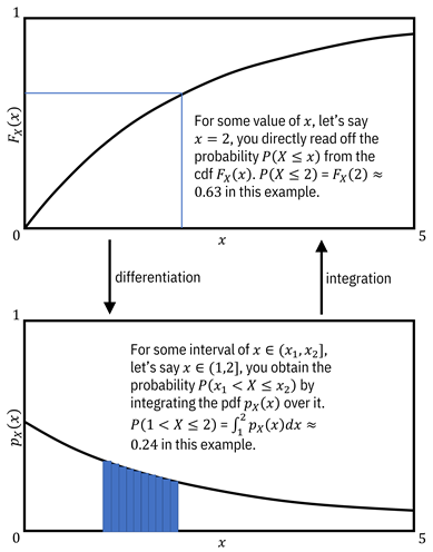
Figure 3.1. An example cdf and corresponding pdf from the ThriveGuild income distribution example. Accessible caption. A graph at the top shows the cdf and a graph at the bottom shows its corresponding pdf. Differentiation is the operation to go from the top graph to the bottom graph. Integration is the operation to go from the bottom graph to the top graph. The top graph shows how to read off a probability directly from the value of the cdf. The bottom graph shows that obtaining a probability requires integrating the pdf over an interval.

Joint pmfs, cdfs, and pdfs of more than one random variable are multivariate functions and can contain a mix of discrete and continuous random variables. For example,  is the notation for the pdf of three random variables , , and . To obtain the pmf or pdf of a subset of the random variables, you sum the pmf or integrate the pdf over the rest of the variables outside of the subset you want to keep. This act of summing or integrating is known as marginalization and the resulting probability distribution is called the marginal distribution. You should contrast the use of the term ‘marginalize’ here with the social marginalization that leads individuals and groups to be made powerless by being treated as insignificant.

The employment status feature and the loan approval label in the ThriveGuild model are random variables that have a joint pmf. For example, this multivariate function could be , , , , , and . This function is visualized as a table of probability values in Figure 3.2. Summing loan approval out from this joint pmf, you recover the marginal pmf for employment status given earlier. Summing employment status out, you get the marginal pmf for loan approval as  and .

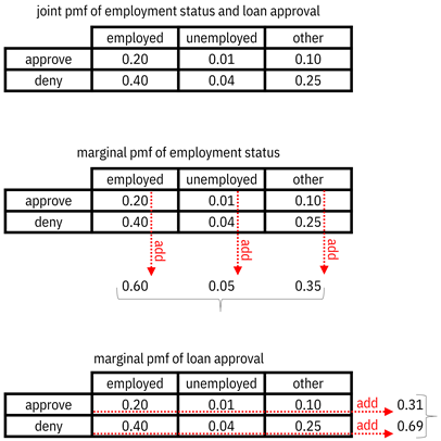
Figure 3.2. Examples of marginalizing a joint distribution by summing out one of the random variables. Accessible caption. A table of the joint pmf has employment status as the columns and loan approval as the rows. The entries are the probabilities. Adding the numbers in the columns gives the marginal pmf of employment status. Adding the numbers in the rows gives the marginal pmf of loan approval.

Probabilities, pmfs, cdfs, and pdfs are all tools for quantifying aleatoric uncertainty. They are used to specify the requirements for the accuracy of models, which is critical for the first of the two parts of safety: risk minimization. A correct prediction is an event and the probability of that event is the accuracy. For example, working with the problem owner, you may specify that the ThriveGuild lending model must have at least a  probability of being correct. The accuracy of machine learning models and other similar measures of basic performance are the topic of Chapter 6 in Part 3 of the book.

3.2.3        Epistemic Uncertainty and Possibility

Aleatoric uncertainty is concerned with chance whereas epistemic uncertainty is concerned with imprecision, ignorance, and lack of knowledge. Probabilities are good at capturing notions of randomness, but betray us in representing a lack of knowledge. Consider the situation in which you have no knowledge of the employment and unemployment rates in a remote country. It is not appropriate for you to assign any probability distribution to the outcomes , , and , not even equal probabilities to the possible outcomes because that would express a precise knowledge of equal chances. The only thing you can say is that the outcome will be from the set .

Thus, epistemic uncertainty is best represented using sets without any further numeric values. You might be able to specify a smaller subset of outcomes, but not have precise knowledge of likelihoods within the smaller set. In this case, it is not appropriate to use probabilities. The subset distinguishes between outcomes that are possible and those that are impossible.

Just like our friend, the real-valued probability function  for aleatoric uncertainty, there is a corresponding possibility function  for epistemic uncertainty which takes either the value  or the value . A value  denotes an impossible event and a value  denotes a possible event. In a country in which the government offers employment to anyone who seeks it, the possibility of unemployment  is zero. The possibility function satisfies its own set of three properties, which are pretty similar to the three properties of probability:

1.    ,

2.    , and

3.    if  and  are disjoint events (they have no outcomes in common; ), then .

One difference is that the third property of possibility contains maximum, whereas the third property of probability contains addition. Probability is additive, but possibility is maxitive. The probability of an event is the sum of the probabilities of its constituent outcomes, but the possibility of an event is the maximum of the possibilities of its constituent outcomes. This is because possibilities can only be zero or one. If you have two events, both of which have possibility equal to one, and you want to know the possibility of one or the other occurring, it does not make sense to add one plus one to get two, you should take the maximum of oneand one to get one.

You should use possibility in specifying requirements for the ThriveGuild machine learning system to address the epistemic uncertainty (reliability) side of the two-part definition of safety. For example, there will be epistemic uncertainty in what the best possible model parameters are if there is not enough of the right training data. (The data you ideally want to have is from the present, from a fair and just world, and that has not been corrupted. However, you’re almost always out of luck and have data from the past, from an unjust world, or that has been corrupted.) The data that you have can bracket the possible set of best parameters through the use of the possibility function. Your data tells you that one set of model parameters is possibly the best set of parameters, and that it is impossible for other different sets of model parameters to be the best. Problem specifications can place limits on the cardinality of the possibility set. Dealing with epistemic uncertainty in machine learning is the topic of Part 4 of the book in the context of generalization, fairness, and adversarial robustness.

3.3           Summary Statistics of Uncertainty

Full probability distributions are great to get going with problem specification, but can be unwieldy to deal with. It is easier to set problem specifications using summary statistics of probability distributions and random variables.

3.3.1        Expected Value and Variance

The most common statistic is the expected value of a random variable. It is the mean of its distribution: a typical value or long-run average outcome. It is computed as the integral of the pdf multiplied by the random variable:

Equation 3.4

Recall that in the example earlier, ThriveGuild borrowers had the income pdf  for  and zero elsewhere. The expected value of income is thus [8] When you have a bunch of samples drawn from the probability distribution of , denoted , then you can compute an empirical version of the expected value, the sample mean, as . Not only can you compute the expected value of a random variable alone, but also the expected value of any function of a random variable. It is the integral of the pdf multiplied by the function. Through expected values of performance, also known as risk, you can specify average behaviors of systems being within certain ranges for the purposes of safety.

How much variability in income should you plan for among ThriveGuild applicants? An important expected value is the variance , which measures the spread of a distribution and helps answer the question. Its sample version, the sample variance is computed as . The correlation between two random variables  (e.g., income) and  (e.g., loan approval) is also an expected value, , which tells you whether there is some sort of statistical relationship between the two random variables. The covariance, , tells you whether if one random variable increases, the other will also increase, and vice versa. These different expected values and summary statistics give different insights about aleatoric uncertainty that are to be constrained in the problem specification.

3.3.2        Information and Entropy

Although means, variances, correlations, and covariances capture a lot, there are other kinds of summary statistics that capture different insights needed to specify machine learning problems. A different way to summarize aleatoric uncertainty is through the information of random variables. Part of information theory, the information of a discrete random variable  with pmf  is . This logarithm is usually in base 2. For very small probabilities close to zero, the information is very large. This makes sense since the occurrence of a rare event (an event with small probability) is deemed very informative. For probabilities close to one, the information is close to zero because common occurrences are not informative. Do you go around telling everyone that you did not win the lottery? Probably not, because it is not informative. The expected value of the information of  is its entropy:

Equation 3.5

Uniform distributions with equal probability for all outcomes have maximum entropy among all possible distributions. The difference between the maximum entropy achieved by the uniform distribution and the entropy of a given random variable is the redundancy. It is known as the Theil index when used to summarize inequality in a population. For a discrete random variable  taking non-negative values, which is usually the case when measuring assets, income, or wealth of individuals, the Theil index is:

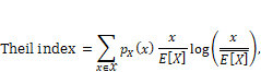
Equation 3.6

where  and the logarithm is the natural logarithm. The index’s values range from zero to one. The entropy-maximizing distribution in which all members of a population have the same value, which is the mean value, has zero Theil index and represents the most equality. A Theil index of one represents the most inequality. It is achieved by a pmf with one non-zero value and all other zero values. (Think of one lord and many serfs.) In Chapter 10, you’ll see how to use the Theil index to specify machine learning systems in terms of their individual fairness and group fairness requirements together.

3.3.3        Kullback-Leibler Divergence and Cross-Entropy

The Kullback-Leibler (K-L) divergence compares two probability distributions and gives a different avenue for problem specification. For two discrete random variables defined on the same sample space with pmfs  and , the K-L divergence is:

Equation 3.7

It measures how similar or different two distributions are. Similarity of one distribution to a reference distribution is often a requirement in machine learning systems.

The cross-entropy is another quantity defined for two random variables on the same sample space that represents the average information in one random variable with pmf  when described using a different random variable :

Equation 3.8

As such, it is the entropy of the first random variable plus the K-L divergence between the two variables:

Equation 3.9

When , then  because the K-L divergence term goes to zero and there is no remaining mismatch between  and . Cross-entropy is used as an objective for training neural networks as you’ll see in Chapter 7.

3.3.4        Mutual Information

As the last summary statistic of aleatoric uncertainty in this section, let’s talk about mutual information. It is the K-L divergence between a joint distribution  and the product of its marginal distributions :

Equation 3.10

It is symmetric in its two arguments and measures how much information is shared between  and . In Chapter 5, mutual information is used to set a constraint on privacy: the goal of not sharing information. It crops up in many other places as well.

 

3.4           Conditional Probability

When you’re looking at all the different random variables available to you as you develop ThriveGuild’s lending system, there will be many times that you get more information by measuring or observing some random variables, thereby reducing your epistemic uncertainty about them. Changing the possibilities of one random variable through observation can in fact change the probability of another random variable. The random variable  given that the random variable  takes value  is not the same as just the random variable  on its own. The probability that you would approve a loan application without knowing any specifics about the applicant is different from the probability of your decision if you knew, for example, that the applicant is employed.

This updated probability is known as a conditional probability and is used to quantify a probability when you have additional information that the outcome is part of some event. The conditional probability of event  given event  is the ratio of the cardinality of the joint event  and , to the cardinality of the event :[9]

Equation 3.11

In other words, the sample space changes from  to , so that is why the denominator of Equation 3.1 () changes from  to  in Equation 3.11. The numerator captures the part of the event  that is within the new sample space . There are similar conditional versions of pmfs, cdfs, and pdfs defined for random variables.

Through conditional probability, you can reason not only about distributions and summaries of uncertainty, but also how they change when observations are made, outcomes are revealed, and evidence is collected. Using a machine learning model is similar to getting the conditional probability of the label given the feature values of an input data point. The probability of loan approval given the features for one specific applicant being employed with an income of 15,000 dollars is a conditional probability.

In terms of summary statistics, the conditional entropy of  given  is:

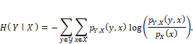
Equation 3.12

It represents the average information remaining in  given that  is observed.  

Mutual information can also be written using conditional entropy as:

Equation 3.13

In this form, you can see that mutual information quantifies the reduction in entropy in a random variable by conditioning on another random variable. In this role, it is also known as information gain, and used as a criterion for learning decision trees in Chapter 7. Another common criterion for learning decision trees is the Gini index:

 

Equation 3.14

3.5           Independence and Bayesian Networks

Understanding uncertainty of random variables becomes easier if you can determine that some of them are unlinked. For example, if certain features are unlinked to other features and also to the label, then they do not have to be considered in a machine learning problem specification.

3.5.1        Statistical Independence

Towards the goal of understanding unlinked variables, let’s define the important concept called statistical independence. Two events are mutually independent if one outcome is not informative of the other outcome. The statistical independence between two events is denoted  and is defined by

Equation 3.15

Knowledge of the tendency of  to occur given that  has occurred is not changed by knowledge of . If in ThriveGuild’s data,  and , then since the two numbers  and  are not the same, employment status and loan approval are not independent, they are dependent. Employment status is used in loan approval decisions. The definition of conditional probability further implies that:

Equation 3.16

The probability of the joint event is the product of the marginal probabilities. Moreover, if two random variables are independent, their mutual information is zero.

The concept of independence can be extended to more than two events. Mutual independence among several events is more than simply a collection of pairwise independence statements; it is a stronger notion. A set of events is mutually independent if any of the constituent events is independent of all subsets of events that do not contain that event. The pdfs, cdfs, and pmfs of mutually independent random variables can be written as the products of the pdfs, cdfs, and pmfs of the individual constituent random variables. One commonly used assumption in machine learning is of independent and identically distributed (i.i.d.) random variables, which in addition to mutual independence, states that all of the random variables under consideration have the same probability distribution.

A further concept is conditional independence, which involves at least three events. The events  and  are conditionally independent given , denoted , when knowledge of the tendency of  to occur given that  has occurred is not changed by knowledge of  precisely when it is known that  occurred. Similar to the unconditional case, the probability of the joint conditional event is the product of the marginal conditional probabilities under conditional independence.

Equation 3.17

Conditional independence also extends to random variables and their pmfs, cdfs, and pdfs.

3.5.2        Bayesian Networks

To get the full benefit of the simplifications from independence, you should trace out all the different dependence and independence relationships among the applicant features and the loan approval decision. Bayesian networks, also known as directed probabilistic graphical models, serve this purpose. They are a way to represent a joint probability of several events or random variables in a structured way that utilizes conditional independence. The name graphical model arises because each event or random variable is represented as a node in a graph and edges between nodes represent dependencies, shown in the example of Figure 3.3, where  is income,  is employment status,  is loan approval, and  is gender. The edges have an orientation or direction: beginning at parent nodes and ending at child nodes. Employment status and gender have no parents; employment status is the parent of income; both income and employment status are the parents of loan approval. The set of parents of the argument node is denoted .

           

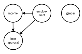
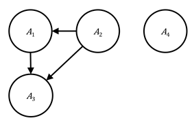
Figure 3.3. An example graphical model consisting of four events. The employment status and gender nodes have no parents; employment status is the parent of income, and thus there is an edge from employment status to income; both income and employment status are the parents of loan approval, and thus there are edges from income and from employment status to loan approval. The graphical model is shown on the left with the names of the events and on the right with their symbols.

The statistical relationships are determined by the graph structure. The probability of several events  is the product of all the events conditioned on their parents:

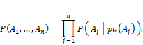
Equation 3.18

As a special case of Equation 3.18 for the graphical model in Figure 3.3, the corresponding probability may be written as . Valid probability distributions lead to directed acyclic graphs. Graphs are acyclic if you follow a path of arrows and can never return to nodes you started from. An ancestor of a node is any node that is its parent, parent of its parent, parent of its parent of its parent, and so on recursively.

From the small and simple graph structure in Figure 3.3, it is clear that the loan approval depends on both income and employment status. Income depends on employment status. Gender is independent of everything else. Making independence statements is more difficult in larger and more complicated graphs, however. Determining all of the different independence relationships among all the events or random variables is done through the concept of d-separation: a subset of nodes  is independent of another subset of nodes  conditioned on a third subset of nodes  if  d-separates  and . One way to explain d-separation is through the three different motifs of three nodes each shown in Figure 3.4, known as a causal chain, common cause, and common effect. The differences among the motifs are in the directions of the arrows. The configurations on the left have no node that is being conditioned upon, i.e. no node’s value is observed. In the configurations on the right, node  is being conditioned upon and is thus shaded. The causal chain and common cause motifs without conditioning are connected. The causal chain and common cause with conditioning are separated: the path from  to  is blocked by the knowledge of . The common effect motif without conditioning is separated; in this case,  is known as a collider. Common effect with conditioning is connected; moreover, conditioning on any descendant of  yields a connected path between  and . Finally, a set of nodes  and  is d-separated conditioned on a set of nodes  if and only if each node in  is separated from each node in .[10]

 

causal chain	connected	separated
common cause	connected	separated
common effect	separated	(or any descendent of  observed) connected

Figure 3.4. Configurations of nodes and edges that are connected and separated. Nodes colored gray have been observed. Accessible caption. The causal chain is  à  à ; it is connected when  is unobserved and separated when  is observed. The common cause is  ß  à ; it is connected when  is unobserved and separated when  is observed. The common effect is  à  ß ; it is separated when  is unobserved and connected when  or any of its descendants are observed.

Although d-separation among two sets of nodes can be checked by checking all three-node motifs along all paths between the two sets, there is a more constructive algorithm to check for d-separation.

1.     Construct the ancestral graph of , , and . This is the subgraph containing the nodes in , , and  along with all of their ancestors and all of the edges among these nodes.

2.    For each pair of nodes with a common child, draw an undirected edge between them. This step is known as moralization.[11]

3.    Make all edges undirected.

4.     Delete all  nodes.

5.     If  and  are separated in the undirected sense, then they are d-separated.

An example is shown in Figure 3.5.

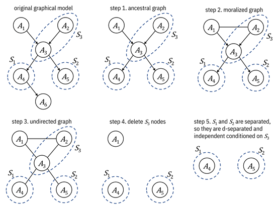
Figure 3.5. An example of running the constructive algorithm to check for d-separation. Accessible caption. The original graph has edges from  and  to , from  to  and , and from  to .  contains only ,  contains only , and  contains  and . After step 1,  is removed. After step 2, an undirected edge is drawn between  and . After step 3, all edges are undirected. After step 4, only , , and  remain and there are no edges. After step 5, only  and , and equivalently  and , remain and there is no edge between them. They are separated, so  and  are d-separated conditioned on .

3.5.3        Conclusion

Independence and conditional independence allow you to know whether random variables affect one another. They are fundamental relationships for understanding a system and knowing which parts can be analyzed separately while determining a problem specification. One of the main benefits of graphical models is that statistical relationships are expressed through structural means. Separations are more clearly seen and computed efficiently.

 

3.6           Summary

§  The first two attributes of trustworthiness, accuracy and reliability, are captured together through the concept of safety.

§  Safety is the minimization of the aleatoric uncertainty and the epistemic uncertainty of undesired high-stakes outcomes.

§  Aleatoric uncertainty is inherent randomness in phenomena. It is well-modeled using probability theory.

§  Epistemic uncertainty is lack of knowledge that can, in principle, be reduced. Often in practice, however, it is not possible to reduce epistemic uncertainty.  It is well-modeled using possibility theory.

§  Problem specifications for trustworthy machine learning systems can be quantitatively expressed using probability and possibility.

§  It is easier to express these problem specifications using statistical and information-theoretic summaries of uncertainty than full distributions.

§  Conditional probability allows you to update your beliefs when you receive new measurements.

§  Independence and graphical models encode random variables not affecting one another.